Query Equivalence

Concept. Two queries are equivalent if they return the same result for ANY input data. They are merely output-equivalent if they happen to agree on the data at hand.

Intuition. Two queries that both return "Mickey, Minnie, Daffy" against today's Listens look identical. Add Pluto with one rating tomorrow, and they may diverge. Real equivalence holds for any input, output equivalence is just today's coincidence.

Important: Query Equivalence vs Output Equivalence

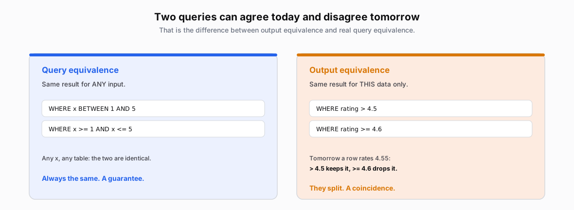
Query equivalence vs output equivalence. Query equivalence (blue): same result for any input, like WHERE x BETWEEN 1 AND 5 versus x >= 1 AND x <= 5; provably the same, a guarantee. Output equivalence (amber): same result for this data only, like WHERE rating > 4.5 versus rating >= 4.6; they agree until a row rates 4.55, then they split, a coincidence.

Running both queries and seeing the same rows only proves they agree on the rows you have. It never proves they agree on the rows you don't. For that you have to reason about what each query computes, as the three examples below do.

Example 1: Users Above Their Personal Average

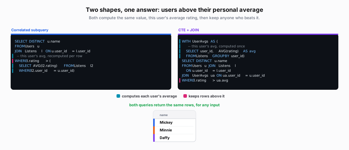
Two equivalent queries side by side (correlated subquery, CTE + JOIN). The teal bar marks where each computes a user's average rating; the pink bar marks where each keeps rows above it. Both produce Mickey, Minnie, Daffy.

Problem: Find users who have at least one rating above their personal average.

Both queries compute the same value, each user's average rating (teal), and keep anyone who beats it (pink). They differ only in when that average is computed: the correlated subquery re-derives it on every row; the CTE computes all of them once, up front. Computing a fixed number once or many times can't change it, so the two are equivalent for any input.

Example 2: Users Who Listen to Multiple Genres

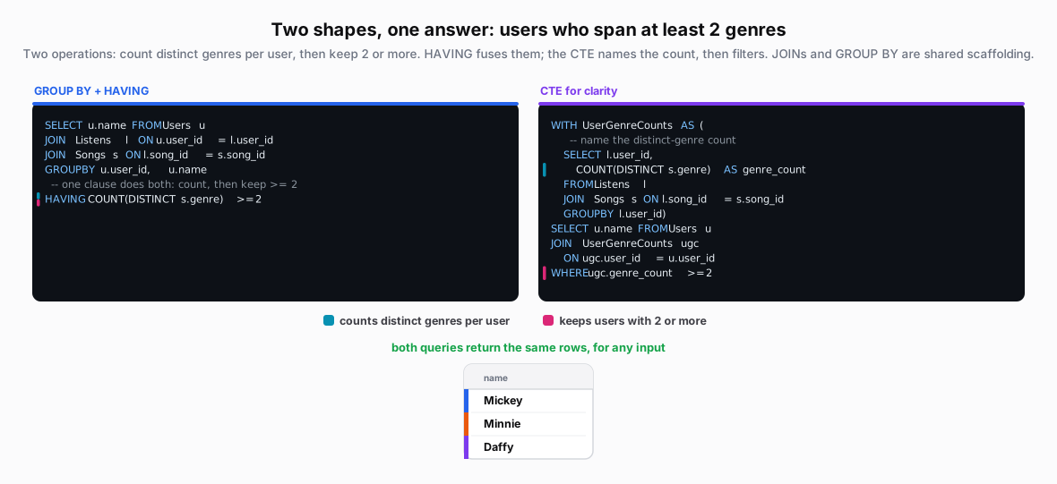
Two equivalent queries side by side (GROUP BY + HAVING, CTE). The teal bar marks where each counts distinct genres per user; the pink bar marks where each keeps users with 2 or more. In the HAVING form one clause does both (a split bar); the CTE names the count first, then filters. Both produce Mickey, Minnie, Daffy.

Problem: Find users who have listened to songs from at least 2 different genres.

The same two operations sit in both queries: count the distinct genres per user (teal), then keep anyone with two or more (pink). HAVING COUNT(DISTINCT s.genre) >= 2 fuses them into one clause, so its role bar is split teal-over-pink; the CTE gives the count a name, then filters on it a step later. The JOINs and GROUP BY are shared scaffolding. Naming a value can't change it, so the two are equivalent for any input.

Example 3: Top 3 Songs per User

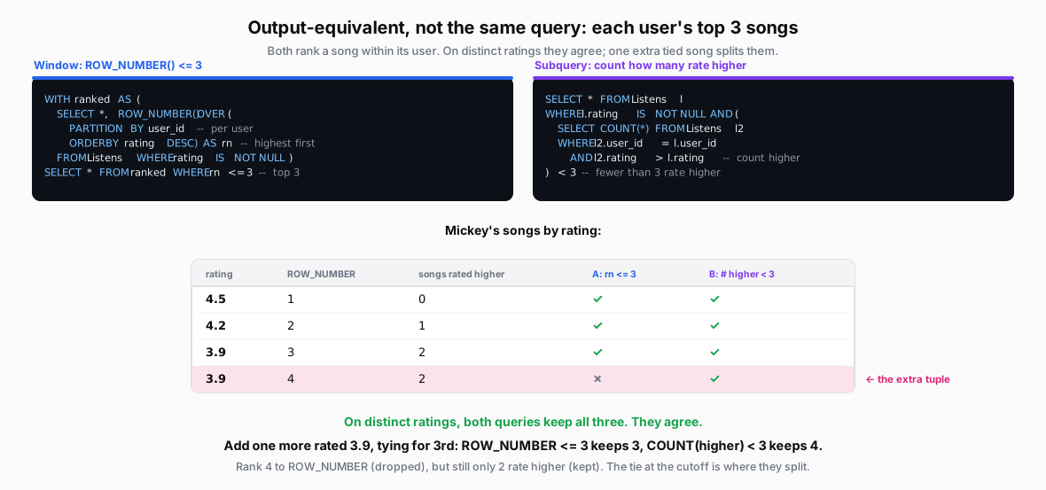
Two queries side by side (window function ROW_NUMBER, classical correlated count) for each user's top 3 songs. On three distinct ratings both keep all three. Add a fourth song tied at 3.9: ROW_NUMBER assigns it rank 4 and drops it (keeps 3), but only 2 songs rate higher so the counting version keeps it (keeps 4). The tie at the cutoff is where they split.

Problem: Find each user's top 3 highest-rated songs.

These two look equivalent and agree on our data, but they are not the same query. Both ask where a song ranks within its user: one with ROW_NUMBER, one by counting how many songs rate higher. On distinct ratings they match. Give one user a second song tied at the cutoff and they split: ROW_NUMBER assigns a strict rank and drops the fourth song, while the counting version still sees only two rated higher and keeps it (see "Where the Look-Alikes Split" below).

Where the Look-Alikes Split

The top-3 pair only looks equivalent: it agrees on our nine rows but splits on a tie. And NOT IN, a pattern you will reach for constantly, hides a related NULL trap. Here are the exact inputs that pull each apart.

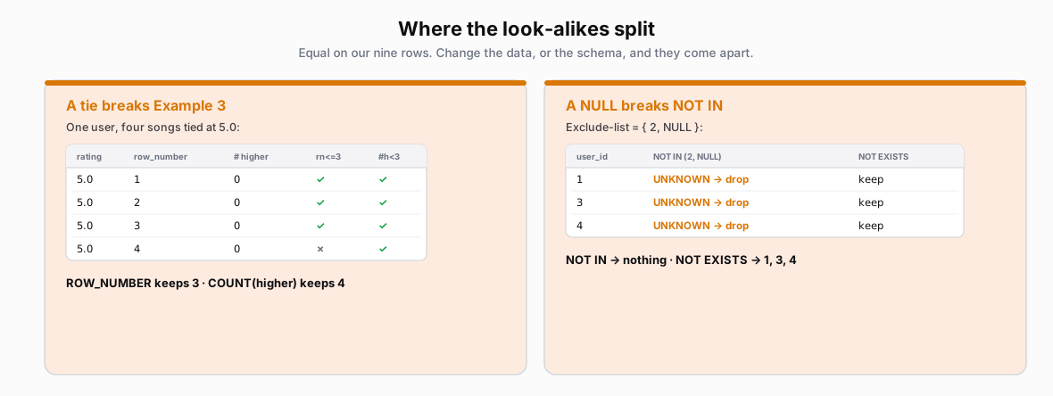
Where the look-alike queries split. With four songs tied at 5.0, ROW_NUMBER keeps 3 rows while COUNT of higher-rated songs keeps 4. With a NULL in the exclude-list, NOT IN returns nothing while NOT EXISTS returns the right rows; on this schema user_id is NOT NULL, so it cannot happen here.

The NULL is the subtle one. NOT IN asks "is this id different from every value in the list?" If the list holds a NULL, you are asking whether a known id differs from an unknown value, and SQL can never answer yes, so the whole result collapses to nothing. NOT EXISTS asks a plain existence question that a NULL cannot poison. On our schema this is blocked, because Listens.user_id is declared NOT NULL. Note that this is the NOT NULL constraint, not the foreign key. A foreign key still permits NULLs; it only requires non-null values to point at a real user.

When to Use Each Approach?

Approach	Best For	Avoid When
Correlated Subquery	• Conceptual clarity • Row-specific logic • Small datasets	• Large datasets • Complex aggregations
CTEs	• Multi-step logic • Reusable calculations • Debugging complex queries • Team readability	• Simple one-off queries • Older SQL versions (pre-2005)
Window Functions	• Rankings (top-N per group) • Running totals • Peer comparisons • Modern SQL environments	• Simple filters • When debugging needed • Older SQL versions
LEFT JOIN + NULL	• Finding non-matches • Performance critical • Complex exclusion logic	• When readability important • Team unfamiliar with pattern
GROUP BY + HAVING	• Simple aggregations • Clear logic • Direct approach	• Need intermediate results • Complex multi-step logic

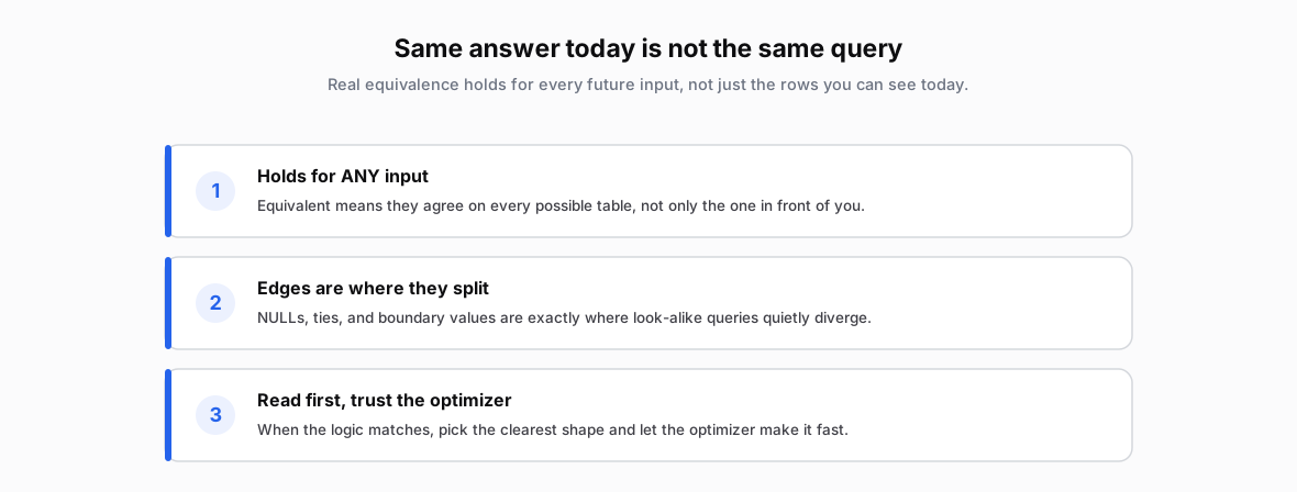
Remember: Prioritize human readability over syntactic cleverness. Trust the query optimizer to handle execution performance.

The Takeaway

Same answer today is not the same query. Real query equivalence holds for any input: equivalent queries agree on every possible table; NULLs, ties, and edge values are where look-alike queries diverge; when the logic matches, pick the clearest shape and trust the optimizer.