Parallel Execution: The Engine Room at Scale
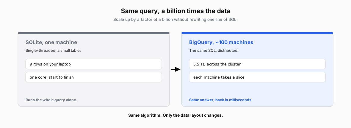
Concept. SQLite and BigQuery run the same hash-join, sort-merge, and aggregate algorithms; they differ in how many machines split the work, not in what work gets done.
Intuition. SELECT user_id, COUNT(*) FROM Listens GROUP BY user_id runs the same hash-aggregate algorithm on the 9-row Listens table in SQLite and on a 5.5-TB Listens table in BigQuery. The big version splits the table across about a hundred machines and runs the same algorithm on each shard.
The Challenge
 Process 5.5 TB of music streaming data to find the top 10 most-played songs since 2024.
The Query
SELECT s.title, s.artist, COUNT(*) AS plays
FROM Songs s
JOIN Listens l ON s.song_id = l.song_id
WHERE l.listen_time > '2024-01-01'
GROUP BY s.title, s.artist
ORDER BY plays DESC
LIMIT 10;
The Journey: From Text to Results in 47ms

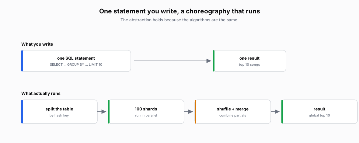
Figure 1. One SQL query over 5.5 TB, about 100 machines, about 47 ms. The engine parses the query into a plan; a coordinator shards the data, runs the same algorithm on every shard in parallel, and merges the partial results. You write what you want; the engine parallelizes the how.
What You're Seeing
Phase 1: Parsing (0-5ms)
The SQL text is tokenized and parsed into an Abstract Syntax Tree (AST). The query optimizer analyzes the AST to determine the most efficient execution strategy based on statistics about table sizes, indexes, and data distribution.
Phase 2: Tree Building (5-12ms)
The logical plan transforms into a physical execution tree. Each node represents a specific algorithmic operation. The tree structure determines the order of operations and data flow. Notice how LIMIT is at the top - we can stop processing once we have 10 results.
Phase 3: Distribution (12-15ms)
The execution tree is decomposed into tasks that can run in parallel. Hash partitioning ensures that related data (same song_id for joins, same grouping keys) ends up on the same machine. This minimizes network traffic during execution.
Phase 4: Parallel Execution (15-45ms)
100 machines work simultaneously, each processing their partition of the data:
-
Green: Join operations matching songs with listens
-
Amber: Group by and aggregation counting plays
-
Purple: Sorting and filtering for top results
Each machine processes one shard, about 55 GB, a split-up slice of the 5.5 TB table, using the same algorithms we'll learn in CS145, distributed across multiple nodes. We cover how this distribution works in the next couple of modules; this page is a preview of how one query breaks into parallel steps.
Phase 5: Result Assembly (45-47ms)
Partial results from all machines converge to a coordinator node. The coordinator performs a final merge-sort to identify the global top 10 songs from the local top results of each machine.
Comparison: Single Machine vs Distributed
| Aspect | Single Machine (SQLite) | 100 Machines (BigQuery) |
|---|---|---|
| Data Size | 9 rows (a few KB) | 5.5 TB (≈55 GB per machine) |
| Execution Time | microseconds | ~47 ms |
| Parallelism | 1 thread | ~800 cores |
| Bottleneck | CPU / memory | Coordination |
| Complexity | Simple | Distributed protocols |
Key Takeaway: Same SQL query on one machine vs 100 machines. Just parallelized.