Locality-Sensitive Hashing and Vector Embeddings
Concept. An ordinary hash spreads similar inputs across different buckets. Locality-sensitive hashing maps similar vectors to the same bucket so a similarity query reads one bucket instead of scanning all vectors.
Intuition. Cut space with a few random lines. For each point, check if the point is above or below each line, and use that as one bit of its code. Two points close together land on the same side of almost every line, so they get the same code and the same bucket. Look only in that bucket.
This is an example of approximation algorithms. Earlier, A Bloom filter answers "is this item in the set?" approximately, accepting a few false positives in exchange for a large space saving. LSH does the same for a harder question, "which items are nearest this one?", accepting a few missed matches in exchange for not scanning a billion vectors.
Locality Sensitive Hashing (LSH)
Every item is a vector in a high-dimensional space, an embedding of hundreds or thousands of numbers. A query is a vector too. "Find similar items" means one thing: of a million stored vectors, which sit nearest the query vector? Comparing the query against all million is O(N), too slow at scale, and an ordinary hash table cannot help: by design it scatters near-identical inputs to unrelated buckets.
 Figure: An ordinary hash scatters similar itemsTwo near-identical cat vectors feed an ordinary hash, which is built to spread inputs out, so they land in unrelated buckets, bucket 7 and bucket 3, far apart in the bucket row. A red bar states the consequence: similar inputs land in unrelated buckets, so finding similar items would have to scan every bucket. This is the problem locality-sensitive hashing fixes. Color key: orange marks the two similar items, grey the hash and buckets, red the two scattered destinations and the verdict.
Figure 1. An ordinary hash spreads inputs across buckets. Two near-identical vectors (cat A and cat B) land in unrelated buckets, 7 and 3. The bucket index carries no information about distance, so a similarity query still scans every bucket. Locality-sensitive hashing groups near vectors instead.
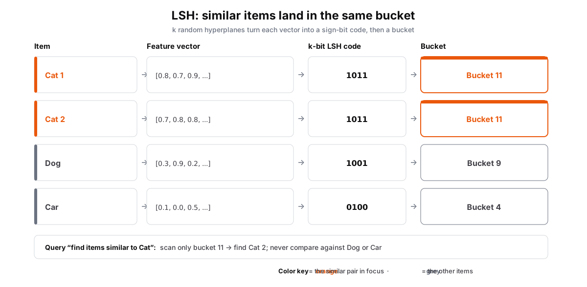 Figure: LSH: similar items hash to the same bucketFour items become feature vectors, then k random hyperplanes turn each vector into a sign-bit code, then a bucket. Cat 1 and Cat 2 are similar so both get code 1011 and bucket 11 (orange, the focus pair); Dog gets bucket 9 and Car bucket 4 (grey). A query for items similar to Cat scans only bucket 11. Color key: orange is the similar pair in focus, grey is the other items.
Figure 2. Each item becomes a feature vector, an embedding, then a short LSH code, then a bucket. The two similar cats receive code 1011 and share a bucket, while the dog and car map to different buckets. A query for items like the cat reads that one bucket instead of comparing against every stored vector. Code bits come from random cuts of the space.
So flip the goal: build a hash that wants collisions, but only between vectors that are alike. Picture one straight line dropped across the space. Every point is on one side of it or the other. In a real embedding space of hundreds of dimensions that line becomes a hyperplane, but nothing else changes: one cut, one yes-or-no question, one bit. We visualize using two figures: the first computes the codes for four items, the second shows what a cut really is once you leave two dimensions.
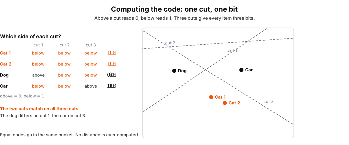 Figure: Each random cut adds one bit to the codeA space crossed by three dashed cuts. Above a cut implies 0, below implies 1, so three cuts give each point a three-bit code. The two cat photos read 111 because no cut falls between them, and share a bucket. The dog reads 011 and the car reads 110. The dog differs on cut 1, the car on cut 3. A table on the left fills in above or below for each point as every cut lands.
| cut 1 | cut 2 | cut 3 | |
|---|---|---|---|
| Cat 1 | below | below | below |
| Cat 2 | below | below | below |
| Dog | above | below | below |
| Car | below | below | above |
Figure 3. Each cut asks one yes-or-no question: above the line is 0, below is 1, and the code assembles one bit at a time. The same four items as Figure 2. The two cats end on 111 because no cut fell between them, so they share a bucket; the dog differs on cut 1 and the car on cut 3, so each lands elsewhere. Nothing measures a distance, so a nearness lookup becomes an ordinary hash-table lookup: cost O(N) drops to about O(N / 2k). Misses happen when a cut does fall between a close pair.
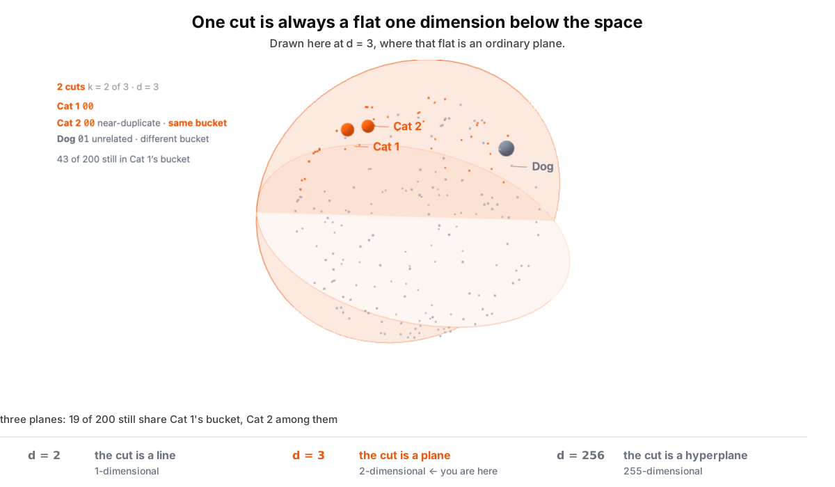 Figure: The cut is always one dimension less than the spaceA cloud of 200 unit vectors in three dimensions, holding the two near-duplicate cats and the unrelated dog. Planes through the origin arrive one at a time and orange marks every vector still on Cat 1’s side of all of them. After the first plane the dog is still in Cat 1’s bucket, because one cut only halves the space; the second plane separates it, and Cat 2 stays throughout. The candidate set falls from 200 to 94, then 43, then 19. A ladder along the bottom names the same object in each dimension: in two dimensions the cut is a line, in three a plane, and in 256 a hyperplane, always one dimension less than the space it cuts.
Figure 3b. A cut is always one dimension below the space it cuts. In 2D that is a line, which is what Figure 3 drew; in 3D it is an ordinary plane, drawn here; in an embedding’s few hundred dimensions it is a hyperplane (hard to picture). Nothing else changes: above or below is still the only question. One cut is insufficient. After the first plane the dog is still in the cat’s bucket, because one cut halves the space and a coin flip put it on that side. The second ejects it, and the near-duplicate survives all three. Each plane roughly halves the candidates: 200, then 94, then 43, then 19.
Why it tracks similarity
A single cut separates two points only when it happens to fall between them. Two close points other leave almost no room for a cut to land between, so nearly every cut puts them on the same side and they keep the same code. Two points further apart leave a wide gap, so many cuts fall between them and flip a bit. The chance two items land in the same bucket therefore shrinks smoothly as they get farther apart. That is what locality-sensitive means: closeness survives the hash instead of being scrambled by it, which is exactly the opposite of an ordinary hash.
The knob: how many lines
Recall measures the fraction of exact nearest neighbours a search returns. For example, if exact search finds the 10 nearest neighbours and an approximate search returns 8 of those 10, its recall@10 is 80%.
More hyperplanes make purer buckets but split more true pairs, so k trades recall for selectivity. You pick k for the recall you need and union several independent tables to recover the pairs any single one drops.
What is Quantization?
LSH shrinks the search. Quantization shrinks the storage: replace each exact value with a small code for the bucket it falls in, so a vector that took kilobytes takes a handful of bytes. Keep just enough to preserve who is near whom. "Find similar" and "store a billion vectors" both become cheap.
Vector/Embedding Hashing
Every large system that searches embeddings runs some version of this: Faiss at Facebook, recommendations at Google and Spotify, semantic and code search at OpenAI. The same locality trick shows up beyond embeddings: perceptual image hashing (Microsoft PhotoDNA) collides near-duplicate images even after a resize or recolor, and DNA k-mer hashing groups similar genomic sequences for fast partitioning. All trade the exact answer for the scale. To see random projections and quantization in working code, open the Hashing Colab.