Case Study 2.1: How Uber and Google Maps index locations
Concept. Uber's H3 and Google's S2 map 2-D coordinates to 1-D cell IDs. H3 uses mostly hexagonal cells, while S2 uses hierarchical quadrilateral cells. This page uses H3 to show how a radius query reads a bounded set of nearby cells before checking exact distances.
Intuition. Compute the H3 cell for every food-delivery order. Nearby orders share a code. At a resolution where one neighboring ring covers 2 km, the candidate lookup reads seven cells instead of scanning 10 million rows.
A radius query checks all 10 million food-delivery orders
A delivery service must group nearby food orders and assign them to drivers quickly. Picture 10 million active delivery orders with coordinates like these:
orders = [(37.788022, -122.399797), (37.788122, -122.399797), (37.788022, -122.398897)]
To find food-delivery orders within 2 km, a naive query evaluates a geo-distance function (e.g,., ST_Distance(driver_loc, order_loc)) across all 10 million rows. It scans the table on every request and can saturate the database during a lunch rush.
A spatial grid narrows the work before the distance calculation. Assign each food-delivery order to a cell, retrieve the cells that cover the search radius, then apply the exact distance check to those candidates. Cell shape and resolution determine how many cells the query reads.
First idea: square cells
Traditional geohashing uses a hierarchical square grid. Each subdivision adds one character to the code. Nearby locations retain a long shared prefix, so a prefix match identifies a neighborhood. At five-character precision, (37.788022, -122.399797) becomes 9q8yy, a cell about 5 km across.
A radius query cannot read only one square because nearby points may lie across a cell boundary. A square has four edge neighbors one cell away and four corner neighbors farther away by a factor of root two. Its first neighboring ring therefore covers distance unevenly.
Why hexagons, not squares
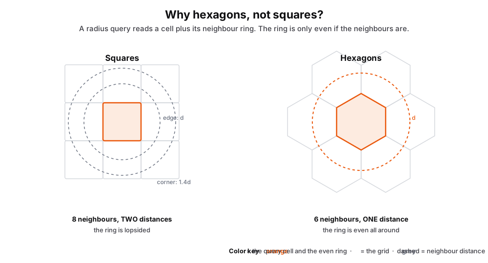 Figure: Why hexagons, not squares: a hexagon's neighbours are all the same distanceTwo grids compared. On the left a square cell has eight neighbours at two different distances: its four edge neighbours are one cell away, its four corner neighbours are farther by a factor of root two, so the ring a radius query must read is uneven. On the right a hexagon has six neighbours, every one exactly the same distance from the centre, so the ring is even in all directions. That uniform neighbour distance is why map systems grid the world into hexagons. Color key: orange is the query cell and, for the hexagon, its single even neighbour ring; grey is the grid; dashed circles are neighbour distances.
Figure 1. Cell shape determines the neighbor ring. A square has eight neighbors at two distances: four edge-neighbors one cell away, four corner-neighbors farther by a factor of root two. A hexagon has six neighbors, each at the same distance from the center, which yields a symmetric ring for a radius query. Hexagons approximate a circle better than squares.
Hexagons give H3 a regular six-cell neighboring ring. Google Maps solves the same indexing problem with S2's hierarchical quadrilateral cells. The worked example below follows Uber's H3 design.
Uber H3: hexagons in practice
Uber's H3 partitions Earth's surface into cells at a chosen resolution (see the H3 and S2 comparison). Higher resolutions produce smaller cells. In this example, three Stanford buildings share a cell at resolution 8 and split into separate cells at resolution 12.
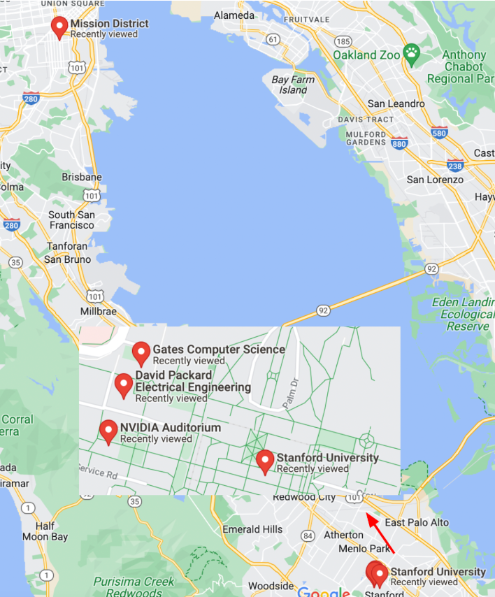
Click to expand. The nearby Stanford pins keep similar H3 codes as resolution changes. The distant SF Mission pin does not.
h3.latlng_to_cell converts each coordinate into an H3 cell ID:
import h3
# lat/lngs from SF mission, Stanford NVidia, Packard, Gates Buildings
locations = [(37.788022, -122.399797), (37.428226, -122.174722),
             (37.429749, -122.1735490), (37.429761, -122.173290)]

for res in [8, 12]:  # H3 resolutions
    for l in locations:
        cell_id = h3.latlng_to_cell(l[0], l[1], res)
        print(f"@res[{res}]: {cell_id}")
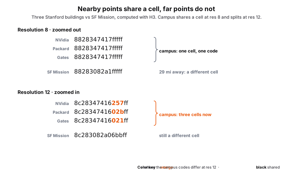 Figure: Nearby points share a cell, far points do notThe three Stanford campus buildings versus SF Mission, computed with H3. At resolution 8 (zoomed out) the three campus buildings get the identical code 8828347417fffff, one shared cell, while SF Mission, 29 miles away, gets a different code. At resolution 12 (zoomed in) the three campus codes split into three cells, differing in the fine digits at the end (orange), and SF stays different. Color key: orange is where the campus codes differ at resolution 12, black is shared.
Figure 2. H3 codes for three Stanford campus buildings and SF Mission. At resolution 8 the three campus buildings map to 8828347417fffff and SF Mission, 29 miles away, maps to a different cell. At resolution 12 the three campus buildings split into three cells, differing in the trailing digits (orange), and SF Mission remains in a different cell.
The hash and the lookup
The index has two stages: map each location to a cell, then retrieve enough neighboring cells to cover the search radius. This produces candidates. An exact distance check removes candidates outside the radius.
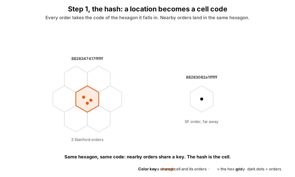 Figure: Geo-hashing: a location becomes a cell codeOrder pins start as raw latitude and longitude. Lay H3's hexagons over the map and every pin falls in one hexagon, which has a cell code. Pins in the same hexagon, three Stanford buildings here, share one code; a far pin in San Francisco gets a different code. The hash is just which hexagon a point lands in. Color key: orange is a shared cell and the pins in it, grey is the hex grid, dark dots are orders.
Figure 3. H3 maps each food-delivery order's latitude and longitude to a cell ID. The system stores 10 million orders by that ID, so nearby orders share one and distant orders fall under different ones.
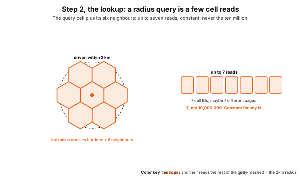 Figure: Geo-hashing lookup: a radius query is a bounded handful of cell readsAt a resolution where one neighboring ring covers two kilometers, the query reads the driver's cell and its six neighbors. Those seven cell identifiers may occupy seven pages. The system then checks exact distances for the candidate food delivery orders. Other radius and resolution combinations may require more rings.
Figure 4. At a resolution where one neighboring ring covers 2 km, the query reads the driver's cell and its six adjacent cells. Those seven cell IDs can map to seven different pages, yielding up to seven reads. The system then checks exact distances for the candidate food-delivery orders. The number of cell lookups stays constant as the table grows from ten thousand orders to ten million; a larger search radius just reads a few more rings.
Takeaway: H3 maps each 2-D location to a 1-D cell ID, so a radius query reads a bounded neighborhood before checking exact distances. In this example, one ring means seven cell lookups instead of a scan over 10 million food-delivery orders.
Video
Play video: 📘 Case Study 2.1: How Uber and Maps use Geo-hashing