Hashing: From Data to Algorithms
Concept. A hash function maps a key to a fixed-size bucket id, so you can find or insert in expected O(1) by reading the page where the bucket lives.
Intuition. Hash-index Listens by user_id, and finding Mickey's 3 listens inside a billion-row table costs one IO, the page where Mickey's bucket lives. No expensive scans.
The bridge from hardware to algorithms
The previous chapter showed why disks and network are slow. From here, the course abstracts those costs into algorithms and data structures:
-
Ignore device-level differences. Reason about IO patterns, not device-level hardware differences.
-
Count IOs. An algorithm that reads 100 pages costs 100 IOs; one that reads a million pages costs 1,000,000 IOs.
So "Algorithm A costs 5N IOs" versus "Algorithm B costs N log N IOs" is a comparison of how many times each hits the disk. Hashing is the first technique that drives that cost down to exactly 1 IO.
Basic Hashing
What is Hashing?
Hashing turns an input of any size into a fixed-size value in [0, B-1]. It is deterministic (same input, same output) and aims for a uniform spread across buckets, giving expected O(1) access. You can't invert the hashed value back into the original input.
Integer Hashing
Simple Modulo Hash
The simplest way to hash integers:
// Simple Modulo Hash
hash_modulo(x, B):
    return x % B
Visual Example: Integer Hashing
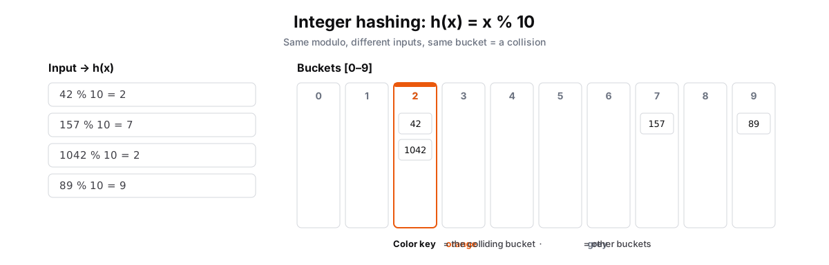 Figure: Integer hashing with h(x) = x % 10Inputs 42, 157, 1042, 89 are hashed by x mod 10 into ten buckets. 42 and 1042 both land in bucket 2, a collision (shown in orange); 157 lands in bucket 7 and 89 in bucket 9. Color key: orange is the colliding bucket in focus, grey is the other buckets.
Figure 1. h(x) = x % 10 maps four integers into ten buckets numbered 0 through 9. 42 and 1042 both land in bucket 2 (orange) because both end in 2, while 157 and 89 fall in distinct grey buckets. The collision is the point: an index must handle two or more keys landing in the same bucket. Chaining stores a list per bucket.
String Hashing
From Characters to Numbers
Strings must first become numbers before they can be hashed. Here's how:
// Simple Sum (Bad - many collisions)
hash_sum(str, B):
    sum = 0
    for char in str:
        sum += ASCII(char)
    return sum % B
A plain sum collides badly (any reordering sums the same). Production code weights each character by a power of a prime so order matters, the polynomial rolling hash in the optional section below.
Hash Collisions
The Birthday Paradox
Just like 23 people in a room make a birthday match likely, hash collisions are unavoidable: a table of B buckets sees a 50% chance of collision after only about √B inserts. Two standard fixes: chaining (a linked list at each bucket) or open addressing (probe for the next empty slot). Keep the load factor n/B under about 0.75 to bound the cost.
Optional: Production-Grade Hash Functions
The simple versions above carry the idea. Real systems mix the bits first, so keys that look alike still scatter across buckets. You do not need these to follow the rest of the course, they are here for reference.
// Integer: MurmurHash-style finalizer (better distribution)
hash_murmur(x, B):
    x ^= x >> 16
    x *= 0x85ebca6b
    x ^= x >> 13
    x *= 0xc2b2ae35
    x ^= x >> 16
    return x % B

// String: Polynomial Rolling Hash (order matters, spreads evenly)
hash_poly(str, B):
    P = 31    // prime number
    hash = 0
    pow = 1
    for char in str:
        hash = (hash + ASCII(char) * pow) % B
        pow = (pow * P) % B
    return hash
Next. Case Study 2.1 applies this exact-bucket hashing to 2-D space: how Uber and Google Maps turn a geo radius query into a one-IO lookup. Then, Locality-Sensitive Hashing, deliberately makes similar items collide so you can search by similarity. See LSH & Vector Hashing.