Case Study 2.3: How OpenAI and Meta's FAISS Speed Up Vector Search
Concept. OpenAI's embeddings are vectors. Meta's FAISS provides exact and approximate indexes for searching them. Vector databases use the same index families (including IVF and HNSW) to avoid comparing a query with every stored vector.
Intuition. An embedding maps content to coordinates, so similar items tend to land near one another. Exact search computes the distance to every stored vector. Approximate nearest-neighbour (ANN) search examines a smaller candidate set, which costs less but may miss the true nearest vector.
The problem: a distance calculation against every row
Anthropic and OpenAI offers embedding models (e.g,, 1,536 or 3,072 dimensions). Take 1,536 as the running example below. One million vectors stored as 32-bit floats occupy about 6.1 GB. An exact nearest-neighbour query compares its query vector with every stored vector. FAISS provides both this exact baseline and approximate indexes that examine fewer candidates.
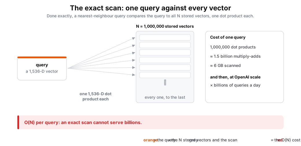 Figure: The exact scan: one query against every vectorExact L2 search computes one distance from the query, a 1,536-D vector, to each of N = 1,000,000 stored vectors, every one to the last. One query costs 1,000,000 L2 distances, about 1.5 billion coordinates and 6.1 GB of vector data, repeated for every query: exact search performs O(N) distance evaluations per query. Color key: orange is the query, grey the stored vectors and the scan.
Figure 1. Exact scan against all N vectors. At one million vectors, a query computes one million 1,536-dimensional L2 distances, covering about 1.5 billion coordinate values and 6.1 GB of vector data. In FAISS, IndexFlatL2 performs this exact search.
The fix: an approximate nearest-neighbour index
Approximate nearest-neighbour (ANN) search gives up the guarantee of returning the exact closest vectors. Its recall and cost depend on the index, the data, and the search parameters. LSH, IVF, and HNSW all examine far fewer than all N vectors:
-
LSH. Random hyperplanes assign vectors to buckets. A query searches vectors in matching buckets.
-
IVF (inverted file). Clustering divides the vectors into cells. A query probes a configured number of nearby cells and skips the rest.
-
HNSW (Hierarchical Navigable Small World). A hierarchy of proximity graphs provides sparse long-range links above denser local links. It often offers a strong recall-latency tradeoff, but the graph consumes memory.
The system builds or updates the index as vectors are added. A query uses that structure to select candidates instead of scanning every vector.
Imagine an HNSW search as a trip from San Francisco to Stanford. You'll try to get to University Ave or Embarcadero or Page Mill, the major arteries near Stanford. Palm Drive does not connect to 101 or 280 directly. In other words, road designers had ``promoted'' a fraction of roads to connect to 101 and 280. You take a freeway for the long part, switch to an expressway, and use local streets near the destination.
That is, the upper graph layers provide long-range links. The bottom layer provides denser local links. The name describes the structure. Hierarchical refers to its layers. Navigable Small World refers to a graph whose local and long-range links support short search paths.
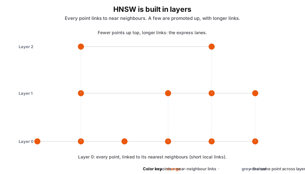 Figure: HNSW is built in layersA hierarchical proximity graph. Layer 0 holds every point with selected nearby links. Random level assignment places fewer points in each upper layer, where links span longer distances. Dashed verticals mark the same point across layers. Color key: orange is points and graph links, grey dashed is the same point across layers.
Figure 2. Each vector is assigned a random height, so only a few rise to the upper layers. At the bottom, nearly all of them connect to their neighbors like local streets. The few promoted higher become the sparse freeway stops the search starts from.
Search starts at an entry point in the highest layer. It greedily moves to closer neighbours, then repeats at each lower layer. At layer 0, HNSW explores a bounded set of candidates and returns the best ones it found. Because the candidate set is limited, the search can miss the true nearest vector.
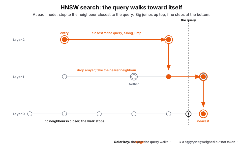 Figure: HNSW search narrows candidates layer by layerThe search starts at an upper-layer entry point, greedily moves toward the query, and descends through the layers. At layer 0, HNSW checks a handful of nearby candidates and returns the best. Color key: orange is the illustrated descent path, the grey ring is a considered neighbour, and the black dashed line is the query.
Figure 3. Top layers are freeways: long links jump you near the query. The bottom layer is local streets: short hops close in. It checks only a handful of candidates, so it is fast but can miss the true nearest.
An index lets a query skip a full scan. You have already built exact hash indexes and approximate LSH indexes. Module 3 covers B+Tree and LSM indexes for keyed lookups. ANN indexes support similarity search.
import faiss
from sentence_transformers import SentenceTransformer

# Demo uses a smaller 768-D model so it runs in a notebook.
# OpenAI's are 1,536-D on the small model, 3,072-D on the large.
model = SentenceTransformer('all-mpnet-base-v2')          # 768-D
strings = [f"String {i}" for i in range(100_000)]
strings[42] = "String 42 is making me hungry"
emb = model.encode(strings).astype('float32')
d = 768
q = model.encode(["String 42 is making me hungry"]).astype('float32')

# Exact baseline: query vs all 100k vectors, O(N) per query
flat = faiss.IndexFlatL2(d)
flat.add(emb)
print(flat.search(q, 5))      # exact, scans everything

# ANN: IVF clusters. Probe only a few of them.
ann = faiss.IndexIVFFlat(faiss.IndexFlatL2(d), d, 256)  # 256 cells
ann.train(emb)                # learns the cluster centroids
ann.add(emb)
ann.nprobe = 8                # probe 8 of 256 cells, skip the rest
print(ann.search(q, 5))       # approximate, far fewer comparisons
Both return String 42 is making me hungry at distance ≈ 0 because the indexed string exactly matches the query. The flat index compares the query with all 100,000 vectors. With nprobe = 8, the IVF index searches vectors assigned to 8 of its 256 cells. The other returned neighbours can differ because IVF search is approximate. You can run this example, and LSH, in the Hashing Colab.
Shrinking the vectors themselves so a billion of them fit in RAM is a separate lever, quantization, and the subject of Case Study 2.4.
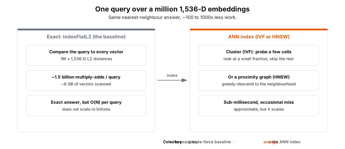 Figure: Brute-force scan vs an ANN indexOne query over a million 1,536-D embeddings. Exact search with IndexFlatL2 compares the query to every vector: one million 1,536-D L2 distances, about 6.1 GB read, an exact answer, O(N) work per query. An ANN index (IVF or HNSW) looks at a small fraction: IVF probes a few clusters, HNSW walks a graph to the neighbourhood. It examines fewer candidates and may miss a neighbour. Color key: orange is the ANN index.
Figure 4. Exact search compares the query with all one million vectors. An ANN index checks only a slice of them, so it answers far faster but can skip the true closest. Check more candidates and you trade speed for accuracy.
Takeaway: OpenAI's embedding models turn content into vectors, and Meta's FAISS provides exact and approximate ways to search them. ANN indexes such as IVF and HNSW examine fewer candidates than an exact scan. Their parameters trade search work for recall. Case Study 2.4 covers quantization, which reduces the memory needed to store the vectors.