IO Cost Summary: Comparing Query Plans
Concept. Add up each plan’s I/O costs. Choose the lower-cost plan.
The cost formulas used here (BigSort, HP, and the three joins BNLJ / SMJ / HPJ, all in terms of C_r, C_w, and page counts P(...)) are the ones defined in Module 3 nanoDB: IO Algorithms. This page uses those formulas and adds them up across a plan.
The Query
-- Count recommendation-listen matches for each song.
SELECT r.song_id, COUNT(r.recommendation_id) AS recommendation_count
FROM Recommendations AS r
-- Goal 1: match the same user and song.
JOIN Listens AS l ON r.user_id = l.user_id AND r.song_id = l.song_id
-- Goal 2: count matching pairs per song.
GROUP BY r.song_id
-- Goal 3: show the largest counts first.
ORDER BY COUNT(r.recommendation_id) DESC;
The Recommendations table. Each row records a song suggested to a user: Recommendations(user_id, song_id, recommendation_id, recommendation_time).
-
Goal 1: Match: join recommendations and listens for the same user and song.
-
Goal 2: Count: count the joined rows for each song.
-
Goal 3: Rank: sort songs by that count, largest first.
A repeated listen counts again. Multiple recommendations for the same user/song also multiply matches. This query does not compare timestamps, so it does not measure whether a recommendation caused a later listen.
A small example
Recommendations
| recommendation_id | user_id | song_id |
|---|---|---|
| 10 | 1 | 497 |
| 11 | 2 | 497 |
| 12 | 1 | 88 |
| 13 | 3 | 75 |
| … | … | … |
Listens
| listen_id | user_id | song_id |
|---|---|---|
| 1 | 1 | 497 |
| 2 | 1 | 497 |
| 3 | 2 | 497 |
| 4 | 3 | 75 |
| 5 | 2 | 88 |
| … | … | … |
Goal 1: Which pairs match?
| recommendation_id | listen_id | user_id | song_id |
|---|---|---|---|
| 10 | 1 | 1 | 497 |
| 10 | 2 | 1 | 497 |
| 11 | 3 | 2 | 497 |
| 13 | 4 | 3 | 75 |
Song 88 has no match: the recommendation is for user 1, but the listen is by user 2.
Goal 2: Count by song
Song 497 has three matches; song 75 has one. These are counts of joined rows, not distinct users.
Goal 3: Largest count first
| song_id | recommendation_count |
|---|---|
| 497 | 3 |
| 75 | 1 |
Query Plan #1: Sort-Merge Join
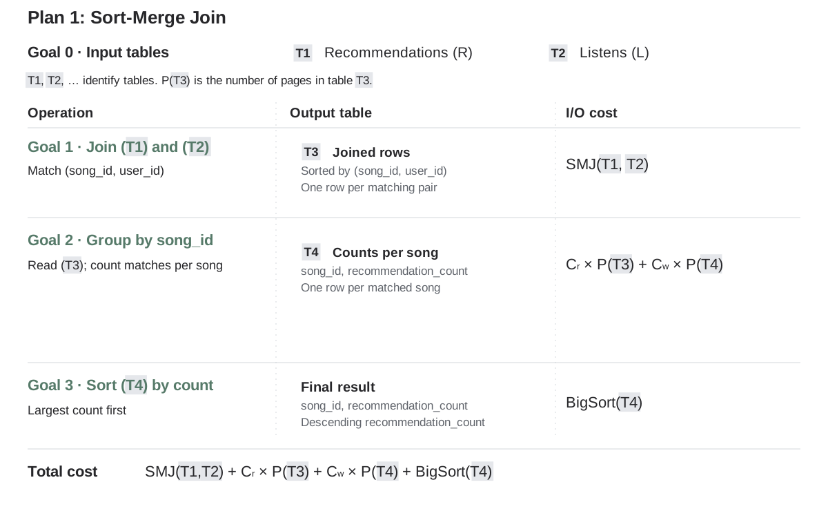 Figure: Plan 1: Sort-Merge JoinGoal 0 identifies input tables 1 and 2. Each following goal shows its numbered output table and I/O cost. Badges identify tables, not row counts.
Figure 1. Sort-merge join leaves rows in song order, so grouping needs no repartitioning.
Query Plan #2: Hash-Partition Join
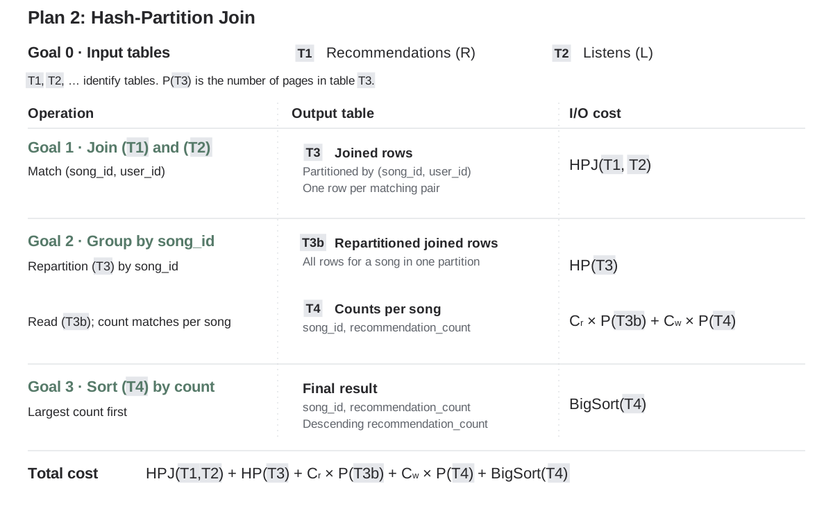 Figure: Plan 2: Hash-Partition JoinGoal 0 identifies input tables 1 and 2. Each following goal shows its numbered output table and I/O cost. Badges identify tables, not row counts.
Figure 2. Hashing by (song_id, user_id) requires a repartition by song_id in this plan.
This plan repartitions by song because hashing the pair does not keep every row for one song together. If all groups fit in RAM, a hash aggregate can avoid this extra partitioning pass.
Compare the two plans
-
Plan 1:
SMJ(T1,T2) + C_r × P(T3) + C_w × P(T4) + BigSort(T4) -
Plan 2:
HPJ(T1,T2) + HP(T3) + C_r × P(T3b) + C_w × P(T4) + BigSort(T4)
Do the math: calculate both total costs and choose the lower-cost plan.