Block Nested Loop Join: The Simple Double Loop
Concept. Block nested loop join loads a block of the outer table into RAM, scans the inner table once per block, and applies the join predicate to candidate row pairs.
Intuition. For a join between a small Songs table and a large Listens table, load Songs into RAM in blocks. For each Songs block, scan Listens and test each listen against each song in the block. Cost: read Songs once, read Listens ⌈P(Songs)/B⌉ times.
The Algorithm: Load Blocks, Scan Everything
A double-for-loop in disguise. Outer loop loads blocks of B pages from the smaller table; inner loop scans the entire larger table for each block; the join predicate fires on every pair.
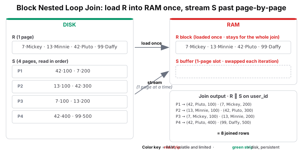 Figure: Block Nested Loop Join: disk inputs, RAM buffers, comparison, and joined outputIn this example R fits in RAM. Load R once into a retained block. Stream S one page at a time into a one-page input buffer. Compare every row in that page with the R block, then emit matching joined rows. Repeat for all four S pages to produce eight rows. Green marks persistent disk; red marks RAM.
Figure 1. Block Nested Loop Join, R ⋈ S. Read the smaller table R from disk and hold it in RAM for the whole join. The larger table S streams past in 4 pages, each loaded into a one-page slot, probed against R, then discarded, producing 8 joined rows (2 per S page here). Best case, when R fits in B pages, is P(R) + P(S) + OUT; if R is bigger than B it becomes P(R) + ⌈P(R)/B⌉ × P(S) + OUT, because S is re-scanned once per R-block. Always make the smaller table the outer one.
BNLJ(R, S, B):                        // R = smaller table (outer), S = larger (inner), B = RAM pages

    // Outer loop: read R one block at a time
    for each block of B pages in R:
        load the block into RAM

        // Inner loop: scan all of S once for this block
        for each page s of S:
            load s into RAM
            for each row r in block, row t in s:
                if r matches t:               // any predicate: equality, range, similarity
                    emit (r, t)
Example: Songs ⋈ Listens
Find all listens for each song. P(Songs) = 100 pages, P(Listens) = 10,000 pages, buffer B = 10 pages. Put the smaller table (Songs) on the outer loop.
| Step | IOs |
|---|---|
| Read Songs once | 100 |
| Blocks of Songs: ⌈100 / 10⌉ | 10 |
| Scan Listens, once per block: 10 × 10,000 | 100,000 |
| Total (plus OUT for the result) | 100,100 |
Compared to a row-by-row nested loop, which rereads Listens once per Songs row (millions of scans), block nested loop is orders of magnitude cheaper just by buffering a block at a time.
Wrong Choice: Listens as Outer
If we used BNLJ(Listens, Songs):
- Blocks: ⌈10,000/10⌉ = 1,000
- Scan Songs: 1,000 × 100 = 100,000
- Total: 110,000 IOs (10% worse)
Non-Equality Joins: Where BNLJ Shines
BNLJ handles any join condition
BNLJ directly evaluates predicates such as:
- Similarity:
similarity(s.features, a.style) > 0.8 - Complex conditions:
s.duration > a.avg_length * 1.5 AND s.genre = a.genre
Real Example: Find Songs Similar to Artist's Style
-- Find songs similar to what the artist usually makes
SELECT s.song_id, a.artist_id
FROM Songs s
JOIN Artists a ON distance(s.audio_vector, a.style_vector) < 0.2
                  AND s.duration BETWEEN a.min_duration AND a.max_duration;

-- Evaluate both conditions for each candidate pair