BigSort: Sorting TBs of Data with GBs of RAM

Concept. BigSort is external merge-sort. It sorts a table larger than RAM by reading RAM-sized chunks, sorting each chunk in memory, writing them back to disk, then merging the sorted chunks together.

Intuition. When you need to sort a 64 GB Listens table by rating on a 6.4 GB machine, read 6.4 GB at a time, sort each chunk in RAM, write each sorted chunk back, then merge the 10 sorted chunks. Cost: read every page once, write every page once, per pass.

How External Merge Sort Uses Memory

External merge sort as a memory model: pages stream from disk (green, persistent) through a small four-page RAM box (red, volatile) and back. Phase 1 reads four pages, quicksorts them, and writes a sorted run; Phase 2 reads the head of each run and emits the smallest, merging into one sorted file. Tiles are pages shaded light to dark by sort key.

Figure 1. External merge sort never holds more than RAM. In Phase 1 it reads four pages into memory, quicksorts them in place, and writes the sorted run back to disk, repeating until the file is a handful of sorted runs. In Phase 2 it reads the head page of each run into memory and emits the smallest value over and over, merging the runs into one fully sorted file. Each tile is a page shaded by its sort key, light for small and dark for large, so a sorted run reads as a smooth light-to-dark gradient. The red box is RAM (volatile), the green is disk (persistent).

Interactive: move every page yourself

Sort 550 values across 58 pages with only a few pages of RAM. Each value is shaded by its rank, so a sorted run reads as a smooth light-to-dark gradient and the raw input reads as noise. Press Play to walk the four stages, or use the tabs to jump between the unsorted input, the Phase 1 sorted runs, and the two merge passes down to one sorted file.

Figure 2. The same sort on real data: 550 values across 58 pages, each shaded by rank. Press Play to watch Phase 1 build sorted runs and the merge passes combine them down to one sorted file.

The BigSort Algorithm (aka External Sort)

Core Idea

Divide: Create sorted runs that fit in memory.
Conquer: Merge those sorted runs into your final output.

Algorithm · BigSort

BigSort(file, B):                 // B = total RAM pages available

    Phase 1: Create sorted runs
    runs = []
    while not EOF:
        chunk = read(B pages)
        sort(chunk)               // quicksort in RAM
        write(chunk to run_i)
        runs.add(run_i)

    Phase 2: Merge runs
    while |runs| > 1:
        next_runs = []
        for i = 0 to |runs| step B:
            batch = runs[i : i+B]     // merge up to B runs per pass
            merged = KWayMerge(batch)
            next_runs.add(merged)
        runs = next_runs
    return runs[0]

Why Sort?

Sorting is the backbone of a database. Every ORDER BY, every range scan on a B+Tree, every sort-merge join, every LSM compaction starts here. PostgreSQL, BigQuery, Spark all run the same operation underneath. Get sort right and the rest of the engine gets fast.

Example Problem: Break Big Sort Into Small Sorts

64GB

Unsorted table

6.4GB

Available RAM

SOLUTION. Apply BigSort to this 10× mismatch: split into 10 sorted runs of 6.4 GB each (Phase 1), then a single 10-way merge combines all 10 runs into the fully sorted 64 GB file (Phase 2). Single merge pass, so cost is 4N IOs total.

Cost Analysis

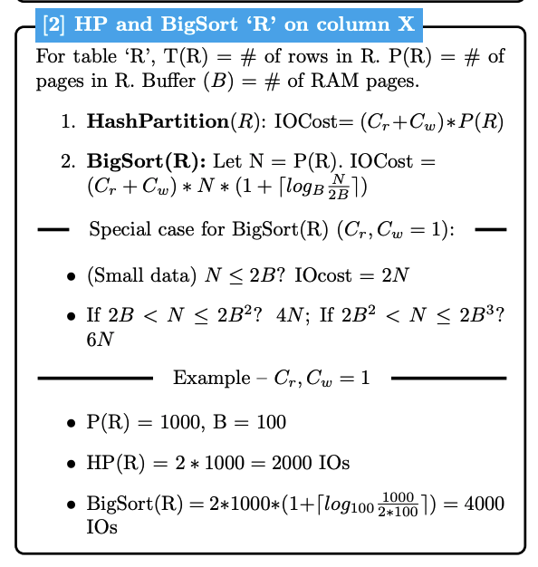
Reference table of per-pass IO costs: BigSort reads and writes every page once per pass at C_r times N plus C_w times N and grows with the number of merge passes; hash partitioning is a flat 2N single pass.

Figure 2. Per-pass IO costs for BigSort against the join algorithms. Each BigSort pass reads and writes every page once, so the cost accumulates one pass at a time as the data outgrows a single merge.

Each pass reads and writes every page once, so a pass costs 2N (C_r×N + C_w×N). Phase 1 builds the sorted runs in one pass; Phase 2 merges, and each merge pass folds up to B runs into one, so it takes ⌈log_B(N/B)⌉ merge passes. The total is 2N × (1 + ⌈log_B(N/B)⌉) — two N times a logarithmic number of passes, so BigSort is O(N log N) in IO, not linear. The familiar 4N is just the single-merge-pass case (small data, where every run fits in one merge); treat it as a best-case approximation, not the general cost. Hash partitioning, by contrast, is a single shot at a flat 2N. The full side-by-side against the join algorithms is on the IO Algorithms page.

In practice: runs of ~2B

The simple version above writes one RAM-sized run per chunk, giving ⌈N/B⌉ runs. Real systems do better with replacement selection: the input streams through an in-memory heap of B pages, and each time the smallest qualifying key is written out, a new page takes its slot. Incoming keys that are still larger than the last one written keep extending the current run, so a run grows to about 2B pages on average instead of B. That roughly halves the run count to ⌈N/2B⌉ and can save a merge pass. The colab and exam cost equations use this ⌈N/2B⌉ form, so an exam cost is 2N × (1 + ⌈log_B(N/2B)⌉).

Sorting is half the big-data toolkit. The other half is the join, and the first join algorithm reuses exactly these RAM-sized blocks.

Block Nested Loop Join → Joining two big tables is the first algorithm that combines everything so far: row access, RAM-sized blocks, and repeated scans.