Optional 6.3c · Big Schemas: What ELT Actually Builds
Concept. A warehouse grows by derivation. ELT loads raw data and runs transformations inside the warehouse, so each transformation becomes a model: one SQL file that contains one SELECT and materializes as a table. Models read other models, so teams stack them into stages. A production pipeline can run eight stages deep. Nine raw feeds can produce forty-two models. The model dependencies form a graph. Lineage names that graph.
Intuition. In this course, each query read Users, Songs, Listens. An insurer's warehouse contains thousands of tables. Each table comes from other tables. The operational question becomes: what is this table made of.
What actually gets big
Module 6.4 ended on a pipeline you have to trust. Start with how much of it there is.
Three tables fit in your head while you learn a JOIN, and every Spotify query you wrote reached straight for one. A real warehouse works the other way round. A few dozen feeds arrive, thousands of tables sit inside, and the ones you query were built in there.
Derivation is the multiplier. Data arrives shaped for the business that sent it, so you reshape it for your question, then reshape the result again.
Healthcare shows why, because no single organisation owns the data. A patient goes in for one visit. A hospital's doctors treat them. An insurer pays the bill. Three organisations, one visit, and each keeps its own record of it. Each names its columns its own way, so the industry agreed on a shared vocabulary: FHIR, which defines each thing as a named resource with a fixed shape.
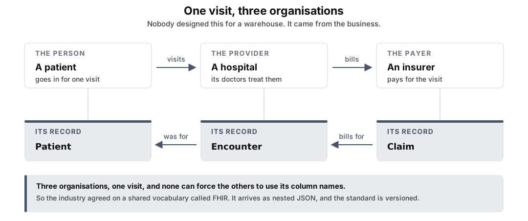 Figure: One visit, three organisationsThe top row tells the real-world story left to right: a person goes in for a visit, a hospital whose providers treat them, and an insurer that pays the bill. An arrow labelled visits joins the person to the hospital, and an arrow labelled bills joins the hospital to the insurer. Below each one sits the record that organisation keeps, named by the FHIR standard: Patient, Encounter, and Claim. Two arrows run right to left between the records, showing that the Claim bills for the Encounter and the Encounter was for the Patient. A band below notes that no party can force the others to use its column names, so the industry agreed on a shared vocabulary that arrives as nested JSON and is versioned.
Figure 1. One visit produces three records in three organisations. FHIR defines dozens more resources. Claim references an Encounter. That Encounter references a Patient. Different companies maintain each record, so references cross company boundaries. The standard changes on a schedule outside your control. The source system chose the format, and the warehouse receives it in that form.
Everyone builds one of these
Nothing in that arrangement is specific to the insurer. The hospital runs its own pipeline, and so does the lab, the pharmacy, and the registry that reports on all of them. Each starts from what its own systems captured, cleans it, combines it, and publishes numbers its own people act on.
The shape repeats. The data does not.
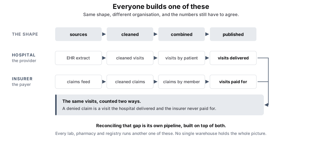 Figure: Everyone builds one of theseA shaded template row at the top shows the shape every organisation builds: sources, then cleaned, then combined, then published. Below it two organisations run their own copy of that shape. The hospital goes from an EHR extract to cleaned visits to visits by patient to a published count of visits delivered. The insurer goes from a claims feed to cleaned claims to claims by member to a published count of visits paid for. A bracket on the right joins both published numbers into one box noting that these are the same visits counted two ways, and that a denied claim is a visit the hospital delivered and the insurer never paid for, so reconciling the gap is its own pipeline. A closing line notes that every lab, pharmacy and registry runs another one, and no single warehouse holds the whole picture.
Figure 2. Two organisations run the same four steps without coordination. The hospital publishes visits delivered. The insurer publishes visits paid for. Both counts describe the same visits and can disagree. A denied or still-pending claim produces a visit the hospital delivered and the insurer did not pay for. Each pipeline can still satisfy its own definition. Another pipeline can reconcile the two by reading both outputs.
Two pipelines can each be right and still disagree, which is why reconciliation is a job of its own. The rest of this page follows one of them. The insurer's is the interesting one, because it is where all three parties have to be joined together.
One job per stage
Module 6.3 settled the choice: ELT lands data raw and transforms it in the warehouse. So a transformation is a SQL file.
That file is called a model. A model is one file containing one SELECT. The tool runs the query and stores the result in the warehouse under the file's own name, so stg_visit.sql produces a table called stg_visit. A file, a query, a table.
Because every model leaves a table behind, the next model can read it. That is how models stack.
One enormous query could go from raw JSON to a readmission rate. Nobody writes one, for the same reason nobody writes one enormous function: you cannot test the middle, reuse a piece, or tell which part broke. So you cut the pipeline into stages, each with one job.
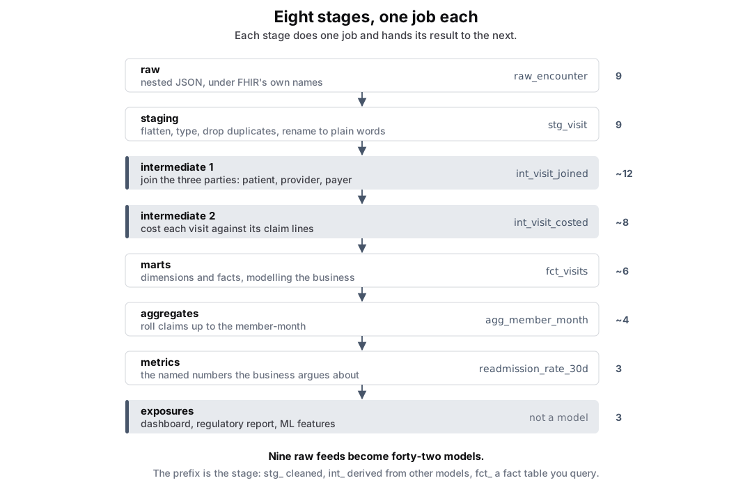 Figure: Eight stages, one job eachA pipeline of eight stages flowing top to bottom, each an equal-width box joined to the next by an arrow. Each box names the stage, says what job it does, shows a real model name from that stage, and carries a count of how many models it holds. Raw lands nine feeds under FHIR's own names, staging flattens and renames them to plain business words, a first intermediate stage joins the three parties, a second costs the encounters, marts build facts, aggregates roll up to the member month, metrics name the numbers, and exposures serve them. A closing line notes that nine raw feeds become forty-two models, and that the prefix on a model name tells you which stage it belongs to.
Figure 3. One build splits into stages. Raw keeps FHIR names chosen by the source. Staging flattens nested JSON, assigns types, drops duplicates, and renames columns to business terms, so raw_encounter becomes stg_visit. Intermediate joins the three parties, then prices each visit from its claim lines. Marts model business entities. Aggregates roll claims up to the member-month because per-claim granularity does not serve reporting. Metrics store named numbers. Exposures are dashboards and reports that read the metrics.
The prefix on a model name is a warehouse convention, and it tells you which stage the model lives in: stg_ has been cleaned, int_ was derived from other models, fct_ is a fact table meant to be queried. Read a name and you know where in the pipeline you are standing.
Each stage does one job and hands its result to the next. The tool knows which model feeds which because you name each dependency as a reference to another model, ref('stg_visit'). The graph gets recorded as you write the pipeline.
The graph nobody drew
Figure 3 summarises the pipeline as eight boxes. Here is every model in it.
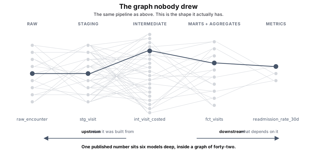 Figure: The graph nobody drewFifty-one models drawn as dots in five columns by stage: nine raw feeds, nine staging, twenty intermediate, ten marts and aggregates, and three metrics. Lines run between adjacent columns and cross heavily. One route is highlighted and named at every step, running from raw_encounter through stg_visit and int_visit_costed to fct_visits and finally the published metric readmission_rate_30d. An axis below marks that walking left is upstream, toward what a model was built from, and walking right is downstream, toward everything that depends on it.
Figure 4. A pipeline is a dependency graph of models. Each dot is a model. Each line is one model reading another. Columns group models by stage from Figure 3. The highlighted route names each step: raw_encounter lands source data, stg_visit cleans it, int_visit_costed joins parties and prices visits, fct_visits shapes the business table, and readmission_rate_30d stores a metric. One route uses six models inside a graph of forty-two.
Every model here is a SELECT a person can read in a minute. The difficulty is distance. readmission_rate_30d sits six models away from the feed it came from, and forty-one other models surround that route.
Walking left from a number is walking upstream, toward what it was built from. Walking right is downstream, toward everything that depends on it. When a number comes out wrong you walk upstream to find the cause: readmission_rate_30d looks wrong, so you check fct_visits, then int_visit_costed, then stg_visit, until the values stop making sense. When you want to change a model you walk downstream to see what you will break: touch stg_visit and everything to its right is in scope.
Takeaway
ELT trades one big transformation for many small ones, and the price of that trade is a graph.
You get a model you can test on its own, a fix that re-runs from raw, and a broken stage that is one file. You also take on more edges than anyone can hold in their head.
The graph is the pipeline, and it is queryable. The day a number goes wrong, walking it is how you find out why. That is 6.3d.
Video
Play video: Optional 6.3c: Big Schemas & Multi-Stage Pipelines