Database Design at Big-Tech Scale
Concept. At big-tech scale, the data stack splits into three systems: OLTP for user-facing writes, OLAP for analytics over billions of rows, and an ETL/ELT pipeline that moves data from one to the other. Heavy analytics do not run on the live OLTP database.
Intuition. A Spotify play writes one row and updates a few counters in Postgres (OLTP). "Top genres this quarter" scans 50 billion rows, so a nightly Spark job ships the data over Kafka to BigQuery (OLAP), where the scan finishes in seconds. The same dataset runs under three latency budgets.
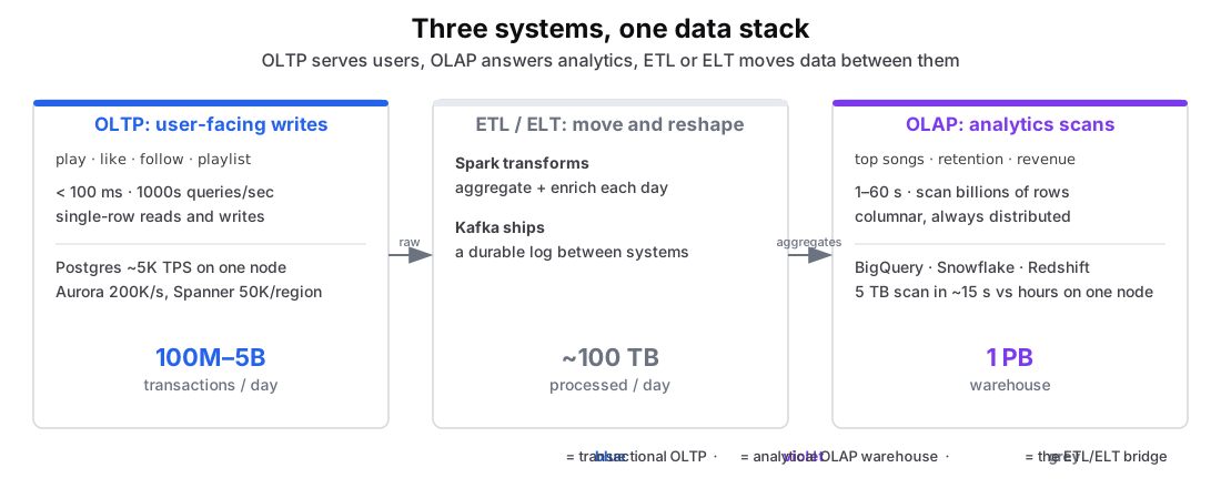 Figure: Three systems, one data stack: OLTP serves users, ETL/ELT moves data, OLAP answers analyticsThree panels left to right. OLTP (blue) handles user-facing writes at low latency on Postgres, Aurora, or Spanner, 100M to 5B transactions a day. ETL or ELT (grey, the bridge in the middle) moves and reshapes data: Spark transforms it and Kafka ships it between systems, about 100 TB a day. OLAP (violet) scans billions of rows for analytics on BigQuery, Snowflake, or Redshift, a petabyte-scale warehouse. Color key: blue is the transactional OLTP system, violet is the analytical OLAP warehouse, grey is the ETL/ELT bridge between them.
Figure 1. One workload split across three systems. OLTP (blue) serves live writes and targets sub-100 ms latency. OLAP (violet) serves analytical scans and reads billions of rows per query. Spark reshapes each day's data and Kafka ships it between the systems. The scale and cost numbers give the order of magnitude for each layer.
Why Not Just One Database?
You pushed startup Postgres to its limit earlier. Eventually a startup becomes an enterprise, and you stop running petabyte-scale analytics on the OLTP system that handles user clicks. The reason is not lock contention: Postgres uses MVCC, so a read-only analytical scan takes no row locks that block writers. The real problem is resource contention at three levels:
-
A long scan saturates CPU and disk I/O, slowing every user-facing query on the same primary.
-
It pollutes the cache, evicting the hot user-facing pages in memory to make room for cold analytical ones.
-
It runs so long that routine cleanup stalls behind it, so the database slowly bloats. (Concretely: the scan holds one read snapshot open the whole time, which keeps
VACUUMfrom reclaiming dead rows.)
So you load raw data into a cheap Data Lake (object storage) and move cleaned slices into an OLAP warehouse built for fast scans over billions of rows.
OLTP: User-Facing Speed
Every click, update, and "add to playlist" is OLTP. A Spotify play:
-- User plays "Anti-Hero" by Taylor Swift
BEGIN TRANSACTION;
INSERT INTO listens (user_id, song_id, timestamp)
VALUES (123, 789, NOW());
UPDATE users SET last_active = NOW() WHERE user_id = 123;
UPDATE songs SET play_count = play_count + 1 WHERE song_id = 789;
COMMIT;
Sub-100 ms latency, thousands of queries per second, single-row updates. One Postgres node handles about 5K transactions/sec for around $500/month; past that you reach for Aurora (200K/sec) or Spanner (50K/sec per region).
OLAP: Analytics at Scale
"What's trending? How are we doing?" is OLAP:
-- Which genres are growing fastest this quarter?
SELECT
    s.genre,
    DATE_TRUNC('week', l.listen_time) AS week,
    COUNT(DISTINCT l.user_id) AS unique_listeners,
    COUNT(*) AS total_plays
FROM listens l
JOIN songs s ON l.song_id = s.song_id
WHERE l.listen_time > '2024-01-01'
GROUP BY s.genre, week
ORDER BY week, unique_listeners DESC;
This scans 5 TB (50 billion rows) in about 15 seconds on BigQuery; on a single Postgres node it would take hours. The reason is parallelism:
1 machine scanning 1 TB:   200 s  (SSD at 5 GB/s)
100 machines in parallel:    2 s  (each scans 10 GB)
Same total work, 100 machines, 100x faster.
ETL/ELT: Moving Data Between Worlds
The pipeline that feeds analytics does three things: Extract from OLTP, Transform (join, aggregate, enrich), and Load into the warehouse. The only open question is the order of the last two, and that order is the whole difference between ETL and ELT.
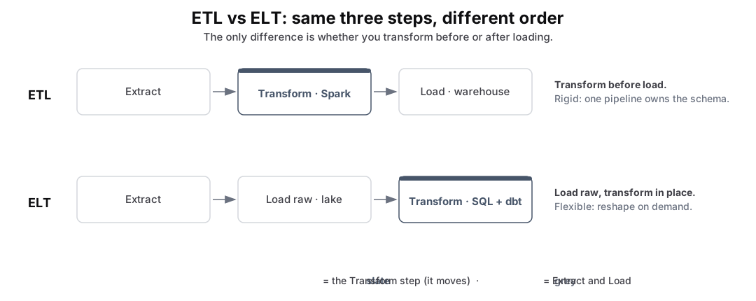 Figure: ETL versus ELT: the same three steps, extract transform load, in a different orderTwo rows. Top row, ETL: Extract, then Transform (slate, the step that moves), then Load into the warehouse, so it transforms before loading. Bottom row, ELT: Extract, then Load the raw data into the lake, then Transform (slate) inside the warehouse with SQL and dbt, so it loads raw and transforms in place. The slate Transform box sits in the middle for ETL and at the end for ELT, so the two steps visibly swap. Color key: slate is the Transform step that changes position; grey is Extract and Load.
Figure 2. ETL transforms before loading. A nightly Spark job cleans and aggregates raw data, then writes finished tables into the warehouse. ELT loads raw data into cheap storage, then transforms inside the warehouse with SQL and dbt. Kafka ships the data in both approaches.
A Spark job for the transform step looks like this:
# Simplified Apache Spark job: aggregate yesterday's plays
from pyspark.sql.functions import count, countDistinct, avg

def spotify_daily_job(spark, songs_dim, users_dim):
    # 1. EXTRACT from OLTP (a PostgreSQL read replica)
    raw_listens = spark.read.format("jdbc") \
        .option("url", "jdbc:postgresql://replica.spotify.com/spotify") \
        .option("query", "SELECT * FROM listens WHERE date = CURRENT_DATE - 1") \
        .load()
    # 2. TRANSFORM: aggregate and enrich
    daily_stats = raw_listens \
        .join(songs_dim, "song_id") \
        .join(users_dim, "user_id") \
        .groupBy("date", "genre", "country", "age_group") \
        .agg(
            count("*").alias("play_count"),
            countDistinct("user_id").alias("unique_users"),
            avg("listen_duration").alias("avg_duration")
        )
    # 3. LOAD to OLAP (BigQuery)
    daily_stats.write.format("bigquery") \
        .mode("append") \
        .option("table", "spotify_warehouse.daily_stats") \
        .option("partitionField", "date") \
        .save()
This job reads from a read replica (not the primary), so the heavy extract never touches the database serving users. Kafka sits between the systems as the durable transport: the transform job publishes its results onto Kafka, and the warehouse, search indexes, and caches all subscribe, so nothing is lost in transit.
The Complete Picture
Users → API → PostgreSQL (OLTP: handle clicks)
                 ↓
              Kafka (carry events reliably)
                 ↓
              Spark (ETL: transform)
                 ↓
            BigQuery (OLAP: answer "what's trending?")
                 ↓
            Dashboards
Key Takeaways
-
Split into three. OLTP for users, OLAP for analytics, ETL/ELT to connect them.
-
Kafka ships the data. A durable log between systems means nothing is lost in transit.
-
It is all SQL. PostgreSQL (OLTP), Spark SQL (ETL/ELT), BigQuery (OLAP).
-
Use the right system per job. Decompose the problem instead of forcing one database to do everything.