Apache Spark: MapReduce Evolved
Concept. Spark generalizes MapReduce by representing a dataset as a Resilient Distributed Dataset (RDD): a partitioned, lazily-evaluated, lineage-tracked collection. You chain many transformations into a single in-memory pipeline that recomputes lost partitions from lineage instead of re-reading from disk.
Intuition. When a data scientist explores last year's Listens with filter(genre == 'pop').groupBy(user_id).count().orderBy(desc('count')).limit(100), Spark builds a single in-memory pipeline across thousands of cores, holds intermediate results in RAM (so the next exploratory query takes seconds, not minutes), and if a machine dies mid-job, Spark recomputes only that machine's partition from the lineage.
RDDs: The In-Memory Pipeline
Spark's core abstraction is the RDD, a Resilient Distributed Dataset. An RDD is the data as it stands after one step, a partial result on the way to the answer. Chain four transformations and you have made four RDDs, three of which are scaffolding. Each one is split into partitions across the cluster and held in memory. Spark records the chain as a lineage graph and evaluates it lazily, in one pass, only when an action finally asks for a result. So intermediate data stays in RAM between stages instead of round-tripping to disk, which is why the same three-stage pipeline (filter to pop, count by user, sort the top) runs about 100× faster than MapReduce.
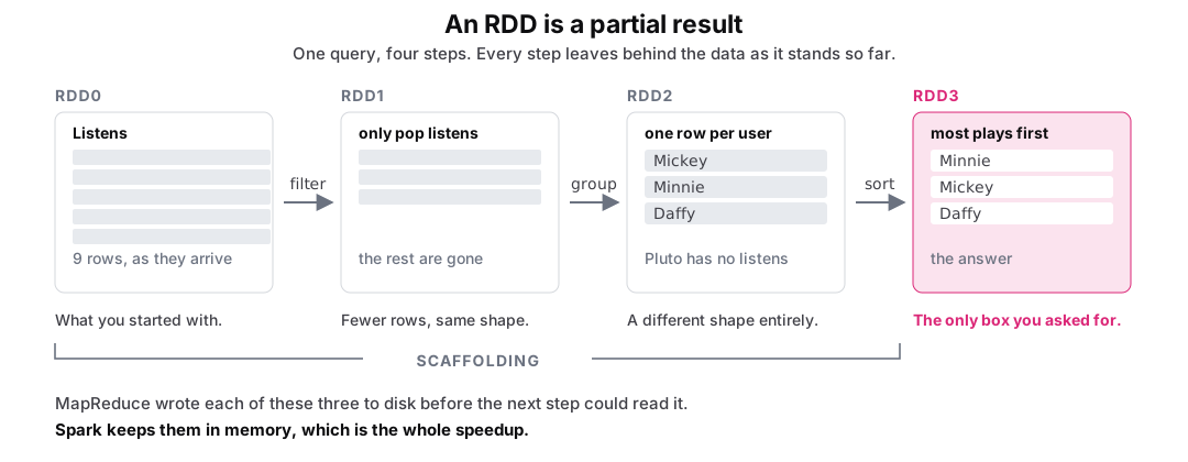 Figure: An RDD is a partial resultFour boxes left to right, each holding a small table, joined by labelled arrows. The first box is RDD zero, the Listens table with nine rows, the data as it arrives. An arrow labelled filter leads to RDD one, the same rows with the non-pop ones gone. An arrow labelled group leads to RDD two, which holds one row per user: Mickey, Minnie and Daffy, with a note that Pluto has no listens and so never appears. A final arrow labelled sort leads to RDD three, the same three users with most plays first. A closing line says each box is the data as it stands after one step, that Spark keeps them in memory rather than writing them to disk, and that the last one is the only box anybody asked for.
Figure 1. One query, four RDDs. Every step leaves behind the data as it stands so far, and only the last box is the answer anybody asked for. The other three are working state. MapReduce wrote each of them to disk so the next step could read it back; Spark keeps them in memory. Pluto never appears after the grouping, because Pluto has no listens.
 Figure: Same multi-stage pipeline: MapReduce writes to disk, Spark stays in RAMTwo panels, same three-stage analytics pipeline (filter to pop, count by user, sort the top). Left, MapReduce runs it as three chained jobs and materializes each job's output to HDFS before the next reads it, about 3 minutes for three disk writes. Right, Spark chains the same three stages into one lazy pipeline that an action triggers and keeps the intermediate RDDs in RAM between stages, about 2 seconds with zero disk writes. The pink elements are the staging medium that sets the speed: the HDFS writes on the left, the RAM pipeline on the right.
Figure 2. The same three-stage analytics pipeline (filter to pop, count by user, sort the top), two engines. MapReduce runs it as three chained jobs and materializes each job's output to HDFS before the next reads it (about 3 minutes); Spark chains the same three stages but keeps intermediate RDDs in memory and evaluates lazily, building a plan it runs once when an action triggers it (about 2 seconds). The ~100× gap comes from data staying in RAM between stages, operator fusion from lazy evaluation, and cheap lineage-based recovery instead of replication.
Resilience: Lineage, Not Replicas
The R in RDD is resilient. RAM is volatile, so if a node crashes mid-job Spark could re-read from disk (slow) or keep three copies of every intermediate (expensive). It keeps the recipe instead: the lineage, which is enough to rebuild any partition on demand.
 Figure: Spark recovers a lost partition by replaying its lineageFour RDD stages left to right: RDD0 input, RDD1 = filter(), RDD2 = map(), RDD3 = map(), each with three grey partitions P0 to P2. These are all narrow transformations, so each output partition depends on exactly one input partition. The worker holding RDD3.P1 dies, so that partition is marked in pink as lost. Spark reads the lineage and re-runs filter then map then map on just the still-alive upstream RDD0.P1, the pink replay path, with no replicas stored.
Figure 3. Spark recovers lost data by replaying lineage instead of keeping replicas. Each RDD records the transformation that produced it (filter, map, map), so Spark stores the operator graph, not the intermediate data. These are all narrow transformations, so each output partition depends on exactly one upstream partition: when a worker dies and takes RDD3.P1 with it, Spark re-runs filter → map → map on just the still-alive RDD0.P1. Storage drops from 3× to 1×, and the cost of a failure rises from reading a replica to recomputing one lost partition. A wide transformation like groupBy would instead re-read every upstream partition through a shuffle.
This works only because Spark's transformations are deterministic: same input, same operator, same output, so replaying the lineage reproduces the lost partition exactly.
Spark SQL: DataFrames + Catalyst
Most teams write SQL or DataFrame transformations rather than low-level RDD code, and Spark's Catalyst optimizer compiles them into the underlying RDD operations.
 Figure: Spark SQL: the same SQL text, executed distributedThe top box holds the Spotify genre-by-week analytics query, a join across listens and songs, identical text to single-node SQL. The lower-left grey box lists Catalyst's execution plan: broadcast the smaller songs table to every node, join it locally against each listens partition, group by genre and week, count distinct users. The lower-right pink box is the payoff: PostgreSQL on one machine takes about 2 hours for 1 TB, spilling to disk on a single node, while Spark on 100 machines finishes in about 3 minutes and scales linearly.
Figure 4. Spark SQL runs the same SQL as Postgres but executes it distributed. The Spotify genre-by-week analytics query (a join across listens and songs) is identical text; Catalyst compiles it to RDD operations: broadcast the smaller songs table to every node, join it locally against each listens partition, then group and count. PostgreSQL on one machine takes hours at 1 TB, spilling the join and sort to disk on a single node with no cluster to parallelize across, while Spark on 100 machines finishes in minutes and scales linearly with cluster size. No code changes between single-node and distributed: the optimizer picks join strategies and partition pruning the same way a single-node optimizer does.
When Spark vs. When MapReduce
Spark wins for:
-
Iterative algorithms. Machine learning, graph processing, anything that touches the same data repeatedly.
-
Interactive analytics. Cached intermediates make follow-up queries return in seconds.
-
Multi-step pipelines. One end-to-end job instead of a chain of separate MR jobs.
-
Mixed workloads. Batch + streaming + ML in one framework.
MapReduce still wins for:
-
Datasets larger than cluster memory. Spark spills to disk when it has to, but if every stage spills, MR's design is the better fit.
-
Single-pass batch jobs. A nightly ETL reads once and writes once, and one pass is exactly the shape MapReduce was built for.
-
Cost-sensitive clusters. RAM is more expensive than disk; when throughput matters more than latency, MR is cheaper.
Spark at Real-World Scale: Netflix Recommendations
Netflix's recommendation pipeline is a join, a grouping and an aggregate. Here it is twice, once in SQL and once as a DataFrame chain, so you can see they are the same query.
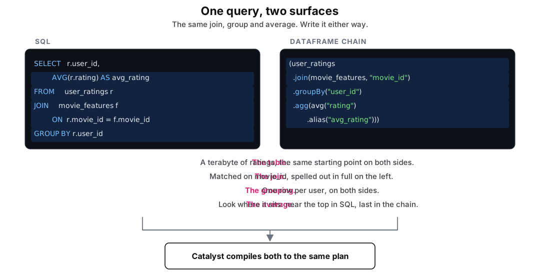 Figure: One query, two surfacesThe same query written twice, side by side on two dark code cards. On the left it is SQL: select r dot user id and the average of r dot rating as avg rating, from user ratings r, join movie features f on r dot movie id equals f dot movie id, group by r dot user id. On the right it is the DataFrame chain: user ratings dot join movie features on movie id, dot groupBy user id, dot agg avg of rating aliased to avg rating. Four highlights walk the two panes together, matching the table, the join, the grouping and the average across both languages. The highlights land on different lines in each pane, because SQL is written in result order while the chain is written in execution order. A closing panel notes that Catalyst compiles both to the same plan.
Figure 5. One query, two surfaces. Read the highlights across: the table, the join, the grouping and the average are the same four operations either way, and Catalyst compiles both to the same plan, so you can write whichever one you prefer. The one real difference is order. SQL puts the average near the top, because it states the result you want; the chain puts it last, because it states the steps in the order they run. Both are lazy, so an action such as show() asks for the rows.
AVG is one aggregate among many. Spark also has array aggregates, and collect_list(rating) is the one you will meet most: instead of reducing a group to a single number, it gathers every value in the group into a list, so one row per user can carry that user's whole rating history. The next step then gets the raw values rather than a summary, which is what handing a group to a model needs.
At the scale this runs:
-
Data: on the order of 1 TB of ratings across 100M+ users
-
Wall clock: minutes rather than the hours the same work took as chained MapReduce jobs
-
Workflow: data scientists iterate interactively instead of waiting overnight
When the Map Step Is a Model Call
Figure 5 was all data work: a join, a grouping, an aggregate. Now put a model in that same chain.
The map in MapReduce was a function you wrote: given a row, return a value. That function can live anywhere, including behind a network call. Databricks' AI Functions put a language model in that slot, and the SQL stays ordinary:
SELECT song_id, title,
       ai_classify(title, ARRAY('workout', 'study', 'party', 'sleep')) AS mood
FROM songs;
One model call per row, a hundred million rows. The driver decides how many calls are in flight and pushes them out across the executors; parallelism, retries and scaling are handled the same way they are for any other stage. None of that changes the engine: the table is partitioned, the plan is lazy, a straggler is still a straggler.
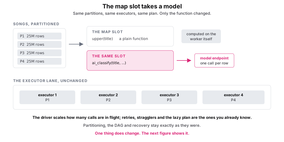 Figure: The map slot takes a modelA Songs table split into four partitions feeds one map slot. First the slot holds an ordinary deterministic function, upper of title, and each partition returns a value computed locally. Then the same slot holds a model call, ai_classify over the title, and each partition instead sends its rows to a model endpoint, drawn in pink. The executor lane underneath is identical in both cases: the same four executors, the same retries, the same lazy plan. A closing line notes that partitioning, the DAG and recovery are unchanged, and only the function in the slot changed.
Figure 6. The slot that held upper(title) now holds a model endpoint, and the engine underneath is unchanged: the same four partitions, the same executors, the same lazy plan and the same retries. Only the function moved off the worker and onto an endpoint. At this scale the hard parts are the ones this module already covers: partitioning, retries, stragglers and cost. The model is the easy part.
One row, or the whole table
Most of these functions are scalar: one row in, one value out, the map step. Three of them read many rows at once, and rows meet in a shuffle.
One row in, one value out
ai_classify · ai_extract · ai_query
Each labels, pulls fields from, or prompts on a single row. This is the map step, so it scales by adding machines.
Many rows in, one answer
ai_forecast · ai_top_drivers · ai_search
One extends a whole time series, one compares two groups, one reads a document set. Each waits on a shuffle, so the shuffle sets the limit.
The open-source engine moved the same way. Spark 4.2 added vector distance and similarity functions and a NEAREST BY clause for top-K ranking joins, which belongs on the shuffle side too: the nearest-neighbour search behind vector indexes becomes a distributed join you write in SQL.
What Breaks: Lineage Meets Non-Determinism
Figure 3 rests on one sentence: replaying the lineage reproduces the lost partition exactly. filter and map keep that promise. A model breaks it.
Ask a model to label the same song twice and you can get two answers. So when a worker dies and Spark rebuilds its partition from lineage, the rebuilt rows can differ from the ones they replaced. The job still reports success. Two rows with identical input can end up with different labels, and which rows differ comes down to which machine happened to fail.
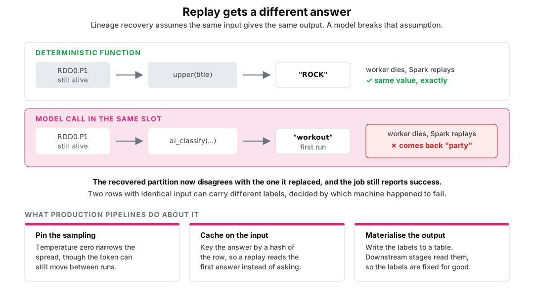 Figure: Replay gets a different answerTwo tracks over the same lineage. On the top track a deterministic function, upper of title, produces the value ROCK; the worker holding it dies, Spark replays the lineage, and the value comes back identical, marked with a green tick. On the bottom track the same slot holds a model call, ai_classify, which first produced the label workout; the worker dies, Spark replays, and the model returns party instead, marked with a red cross, so the recovered partition disagrees with the one it replaced. A closing panel lists the three fixes used in practice: pin the sampling to temperature zero, cache the answer against a hash of the input row, and materialise inference output to a table, which fixes the labels for good.
Figure 7. The same recovery that makes Spark cheap makes a model pipeline inconsistent. Production pipelines close the gap three ways, and only the last one closes it completely: temperature zero narrows the spread while the token can still move; caching the answer against a hash of the input row makes a replay read rather than ask; and materialising inference output to a table removes recomputation entirely, so real pipelines write predictions down once and read them after that.
Determinism was a footnote as long as the map step was arithmetic. Put a model in that slot and it becomes the design constraint.
Key Takeaways
-
Same primitives, better execution. Spark uses the same hash partitioning and worker model as MapReduce. The change is keeping intermediate data in RAM and tracking lineage.
-
Memory-centric design unlocks new workloads. Iterative ML, interactive analytics, and large-scale graph processing become tractable when intermediate state lives in memory.
-
One framework, many APIs. Spark Core (RDDs) → Spark SQL (DataFrames + the Catalyst optimizer) → Spark Streaming → MLlib. Same execution engine, different surfaces.
-
Determinism enables lineage. Spark's fault-tolerance trick only works because every transformation is deterministic. Replay produces the same result, and a model in the map slot breaks that promise.