Distributed Sort & Hash
Concept. Distributed sort and hash are the two foundational data-movement primitives in a cluster: hash partitioning routes every row with the same key to the same machine (so joins and group-bys can run locally), and distributed sort puts the whole dataset in order across the cluster, each machine holding one contiguous key range, so per-key reductions can stream.
Intuition. When Spotify wants to count "lifetime listens per user" across a year of play logs, hash-partitioning by user_id sends every event for Mickey to the same node, every event for Minnie to another, so each node can sort its own subset and emit (user_id, count) pairs without ever talking to peers about other users.
Distributed Sort: One Total Order Across Machines
The first primitive puts the entire dataset in order across the cluster, in three passes: each machine sorts locally, the cluster samples split points, and rows redistribute so the machines line up end to end.
 Figure: Distributed sort in three phasesThree machines sort a dataset into one global order in three phases. Phase one: each machine sorts its own partition locally. Phase two: the cluster samples the data to pick two split points that divide the value range into thirds. Phase three: machines redistribute rows by split point, so node one holds the lowest range, node two the middle, node three the highest, a total order across the cluster.
Figure 1. Distributed sort in three phases. Each node first sorts its own partition locally. The cluster then samples the data to pick split points that divide the value range into equal pieces (here ≤3, 4 to 6, ≥7). Finally rows redistribute so each node owns one contiguous range, and reading the nodes in order gives a single total sort. Sampling is what keeps each node's share balanced even when the data is skewed.
Hash Partitioning: Foundation of Distribution
The Core Problem
When your dataset outgrows RAM, you split it across machines. Hash partitioning keeps related data together: it sends every row for one key to one machine, so a user's events never scatter between Ohio and Tokyo.
The Payoff: a Distributed Join
A join runs locally when both inputs are partitioned on the join key. Hash both tables on that key (here user_id), and every row for a given user_id, from either table, lands on the same machine. Each machine joins only its own slice, and the parts union into the full result.
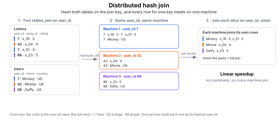 Figure: Distributed hash join: hash both tables on the join key user_id, so every row for a user_id meets on one machine, then join locallyThree stages left to right. First, two tables joined on user_id: Listens (user_id, song_id, rating) and Users (user_id, name, country), with rows colored by the user_id value (7 blue, 42 orange, 88 purple). Second, both tables are hashed on user_id, so every row with a given user_id, from either table, is routed to the same machine: user_id 7 to machine one, 42 to machine two, 88 to machine three. Third, each machine joins only its own slice on user_id and the partial results are unioned into the full join. No machine compares its rows against another machine's, so throughput scales with the cluster.
Figure 2. A distributed hash join. Both tables are hashed on the join key user_id, so every row for one user_id, from either table, is routed to the same machine (the colour is the key value: 7 blue, 42 orange, 88 purple). Each machine joins only the rows it holds, then the partial results union into the full join. No machine compares its rows against another machine's, so throughput scales with the cluster.
Consistent Hashing
The Problem: Adding/Removing Machines
Standard hashing (machine = hash(key) % N) reshuffles almost everything when you change the machine count:
-
From 3 to 4 machines: about 75% of data moves.
-
From 100 to 101 machines: about 99% of data moves.
The Hash Ring
Replace modulo with a ring:
-
Create a ring: Numbers 0 to 2³²-1 form a circle.
-
Place machines on the ring:
hash(machine_id)determines their spot. -
Place keys on the ring:
hash(key)finds their position. -
Key ownership rule: Move clockwise from a key until you hit a machine, that's its home.
 Figure: Consistent hashing: each key goes to the first node clockwise, and adding a node moves only the small arc behind itA ring spans 0 to 2^32 minus 1. Three grey nodes A at the top, B lower right, C lower left, sit at hashed positions. Three grey keys sit on the ring, and from each a pink arrow walks clockwise to the first node it meets. Then a new node D is added halfway between C and A. Only the keys in the short green arc between C and D move: key 1 leaves A and goes to D. Key 2, which sits past D between D and A, still walks clockwise to A and does not move; nor does key 3. So adding a node shifts only that one small arc, about 1 over N of the keys, not the whole side.
Figure 3. Consistent hashing places both keys and machines on a ring over 0 to 2³²−1; each key belongs to the first node clockwise from it. A new node steals only the keys between it and its predecessor, about 1/N of them, so the cluster grows without the near-total reshuffle hash % N forces. DynamoDB, Cassandra, memcached pools, and CDN load balancers all run on this.
Key Takeaways
1. Hash Partitioning
The backbone of distributed processing
-
Keeps all rows with the same key on one machine.
-
Runs joins and group-bys in parallel without cross-talk.
-
Cost: 2N IOs (one read, one write).
-
Scales to hundreds of machines.
2. Distributed Hash Joins
Scaling joins
-
Route both tables by the join key.
-
Each machine joins its local partition.
-
Union the local results for the full join.
-
More machines give linear speedup.
3. Consistent Hashing
Scaling without a full reshuffle
-
Maps keys and nodes to a ring instead of modulo.
-
Adding a node only touches its immediate neighbors.
-
On average only K/N keys move, versus K keys with standard hashing.
-
Used by Cassandra, DynamoDB, Memcached.
4. Distributed Sort (BigSort)
Total order across the cluster
-
Phase 1: each machine sorts its own partition.
-
Phase 2: sample the data to pick global split points.
-
Phase 3: redistribute by split point and finalize.
-
The result is a total order across the cluster.