Build NanoMem, a retrieval engine with keyword search, vector search, and hybrid retrieval. Index CodeSearchNet Python functions [~450k functions] and MS MARCO v1 web passages [~8.8 million passages]. Compare your results and query times with SQLite FTS5 and sqlite-vec. At higher tiers, handle data larger than your memory budget.
What industry is building: Coding assistants search code and documentation to answer requests such as “Where is session expiration handled?” NanoMem builds the retrieval layer behind that search. See the kickoff case study, Claude & OpenAI: Deconstructing Agent Memory.
What you will learn: In Phase 0, set up a basic retrieval prototype using SQLite and collect baseline benchmark results. From Phase 1 onward, build your own indexes and retrieval methods, measure when each works well, and explore how partitioning trades memory for disk reads.
Implementation rules: Write the retrieval algorithms yourself. Use SQLite as the baseline and comparison, not as your NanoMem engine. Library and AI policy.
Figure: From a SQLite baseline to your own NanoMem enginePhase 0 uses SQLite FTS5 and sqlite-vec to establish baseline results. A dotted vertical line separates it from Phases 1 through 6: implement a query planner, retrieval, ranking, and results, then benchmark against SQLite.Figure 1. From baseline to NanoMem. Phase 0 runs the supplied SQLite prototype. In Phases 1–6, build your engine and compare it with the same SQLite references.
Requirements and resources
Proposal: Oct 30 (10 points; no late days)Final: Nov 20 (90 points; late-day policy)
Phase 0: Proposal and baseline prototype setup
Run the supplied baseline prototype on tiny data (1,000 Python functions and 1,000 web passages). The starter loads the data, creates embeddings, and runs SQLite FTS5 and sqlite-vec.
Inspect the keyword and vector-search results. Later, you’ll build your own NanoMem engine and keep SQLite as the comparison baseline. No NanoMem implementation is required for the proposal.
Run the proposal-size data (DATASET = "25k": 25,000 documents per dataset), then complete the proposal checklist.
Core work: Implement keyword, vector, and hybrid retrieval. Compare all five methods with SQLite references. See What to implement and the Library and AI policy.
Grading: Required work earns phase points (larger scale within the memory limit unlocks more points).
Submit: One executed notebook with saved tests, benchmarks, and the Phase 6 writeup.
Resources
Important: Optional checkpoints (Phase 1 onward). Uncomment and run the Drive checkpoint code after Setup to save files written to the checkpoint folders in your Google Drive. Recommended for longer runs; not required for Phase 0.
For coding: Download the notebook, then open it in Colab with File → Upload notebook. Local Jupyter also works; no paid subscription required.
Runtime: Run locally on your computer (including a Mac) or in Colab. CPU works; a supported GPU can speed up embeddings. In Colab, choose Runtime → Change runtime type → GPU if available. The starter defaults to CPU: set EMBED_DEVICE to "cuda" for a Colab/NVIDIA GPU, or "mps" for a supported Mac GPU.
Teams: Two students recommended; solo allowed. One submission per team. Late days are deducted from both partners and limited by the smaller remaining balance. See the partnership and late-day policy.
Grading
What to implement
Complete Phases 0–6 below (100 points total). This page contains the requirements and grading; the notebook contains implementation cells, function contracts, and tests.
Phase
Section
Points
0
Run FTS5 and sqlite-vec on both proposal datasets. Submit the Phase 0 proposal by Oct 30; late proposals earn no Phase 0 credit.
10
1
Implement the inverted index and BM25; pass the supplied tests. Compare Recall@5 with FTS5 using identical data and queries; investigate quality gaps and explain your design choices.
20
2
Implement LSH and pass its tests. Compare Recall@5 with sqlite-vec using identical data and queries; investigate quality gaps and explain your speed/recall tradeoffs.
20
3
Implement RRF hybrid retrieval, a query planner, and a custom fusion method. Pass the fusion and routing tests; explain your custom method. It need not beat RRF.
15
4
Benchmark five methods on both datasets: BM25, LSH, RRF hybrid, custom fusion, and planner-routed retrieval. Return 10 results per query when available. Use identical evaluation queries and report recall, MRR@10, latency, and memory.
10
5
Add FTS5 and sqlite-vec to the same comparison using identical data and queries. Reuse Phase 4 results.
10
6
Write half a page to one page: findings (5), 2–3 AI-use examples and how you checked them (6), and a plain-English explanation of one algorithm (4). If you choose not to use AI, describe 2–3 debugging or design decisions and how you tested them instead. Figures, code, and benchmark tables do not count toward the page limit.
15
Total
100
Keep the supplied tests and save full-scale results. Passing tiny-data tests alone does not establish full-scale correctness. Show examples of missed results when investigating quality gaps. There is no fixed recall-gap cutoff. Use the notebook’s function contracts for implementation details.
What to index and how it’s scored
Run your implementation at the scale below. Your demonstrated tier sets the maximum base score. Tier 87 is the recommended target. State your target in the proposal; you may change it later.
Tier 80 · 25K documents per datasetReport memory use; no memory cap.
Complete the shared phase rubric above using DATASET = "25k": 25,000 Python functions from CodeSearchNet’s training split and 25,000 web passages from MS MARCO v1.
Tier 87 · 250K documents per datasetRecommended target. Report memory use; no memory cap.
Use DATASET = "250k": 250,000 Python functions from CodeSearchNet’s training split (412,178 available) and 250,000 web passages from MS MARCO v1. Submit results for both datasets. The implementation and phase rubric are unchanged.
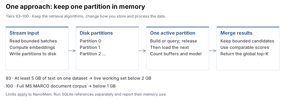
Tier 93 · Tier 87 runs + at least 5 GB of text on one datasetBuild and query with a working set below 2 GB.
Keep both Tier 87 runs and add the supplied fixed MS MARCO v1 document subset: 709,254 documents containing 5 GB of title/body text. The Setup utilities provide the loader; call it in the notebook’s Tier 93 section. Everyone uses the same documents and queries. Save your indexes to reuse for the optional bonus. These are full web documents, rather than the starter’s shorter passages.
Additional implementation: Build and query within the memory budget. Incremental loading, disk partitions, and bounded query merging are suggested approaches; no separate streaming framework is required. The supplied smaller-dataset loaders hold documents in memory, so adapt or replace them for this run.
Measure: live memory during building and querying, including embedding batches, shared state, and temporary buffers. The limit applies even on larger machines. Run SQLite references separately; report their memory, but they need not meet this cap.
Evaluate: use the supplied 50 development queries and 500 separate final queries and their relevance labels. Use the same final set for all five methods and both references. Do not tune on the final set.
Measure UTF-8 document-text bytes before compression; exclude embeddings, indexes, and padding duplicates. Use decimal GB. Report text and embedding bytes separately.
Figure: One approach: keep one partition in memoryStream documents and embedding batches into disk partitions. Build and query one partition at a time, retaining bounded candidates for a global merge. Tier 93 uses at least 5 GB of text under a 2 GB live working set; Tier 100 uses the full MS MARCO v1 document corpus under 1 GB.Figure 2. Scale with bounded memory. Measure the tradeoff between live memory, disk reads, and query time.Tier 100 · Tier 93 runs + full MS MARCO document corpusWorking set below 1 GB.
Expand the Tier 93 subset to the full MS MARCO v1 document-ranking corpus (3,213,835 documents). Keep your earlier results. Additional implementation: Build and query the full corpus with a working set below 1 GB. Use the same memory accounting as Tier 93.
Evaluate: reuse the saved Tier 93 development and final query sets and their relevance labels. Compare all five methods and both SQLite references on the full corpus. Do not tune on the final queries.
Show: measured title/body text size, document count, benchmark results, memory evidence, and disk reads. The published 22 GB TSV size includes metadata; report your actual indexed text size.
Before larger runs, measure runtime and disk needs on a small subset.
Grading and partial credit: Phase 0 is worth 10 points. Your tier caps the final submission at 70, 77, 83, or 90 points. We award partial credit for the work demonstrated; a missing proposal earns 0/10.
Optional bonus:
Run: Use the optional benchmark code in the notebook, reusing your Tier 93 data and indexes.
Save: Keep the benchmark results in your submitted notebook. No separate attachment is needed.
Review: Staff review the results and finalize the awards; the top five valid entries receive 0–5 extra points.
Metrics for your required benchmark runs
Report these metrics for the runs specified by your tier. T93 includes the T87 runs; T100 keeps those results and adds the full-corpus run.
Benchmark note: CodeSearchNet queries come from docstrings included in the indexed functions, so keyword matching has an advantage. Compare your implementation against its corresponding SQLite baseline; vector search need not outperform keyword search.
R@1, R@5, R@10
Recall at K. The fraction of known relevant documents retrieved in the top 1, top 5, or top 10.
Averaged over all eval queries. Higher is better; 1.0 is perfect.
MRR@10
Mean reciprocal rank. 1 / (rank of the first relevant answer within the top 10), averaged. A query scores 0 if none of those results is relevant.
Higher scores mean the first relevant result appears earlier.
p50, p95 ms
Latency. Median and 95th percentile query time in milliseconds.
Peak memory and working set
Two related numbers.Peak RSS (resident set size,
via psutil) is the largest resident-memory measurement sampled during the run.
Working set is what's live in memory at any one moment, which is
what we grade against the 2 GB and 1 GB targets at Tier 93 and Tier 100.
At Tier 80 and Tier 87 you just report both numbers, no cap. See
Tier 93 FAQ for what to keep visible in your
notebook so we can verify residency without re-running.
What to submit
Submit both deliverables through Gradescope. Keep the required outputs visible in your notebook.
Proposal · Oct 30
After the tiny-data check, set DATASET = "25k" (25K documents per dataset) and rerun Phase 0 for the proposal.
Submit the same notebook with Phase 0 executed and its proposal summary filled in by October 30 (course Week 6). Phase 0 is worth up to 10 points. No late days are allowed for the proposal.
Query results: for each proposal dataset, run the supplied query and two variants you write using both keyword and vector search. Keep the three ranking tables visible, including query text, document IDs, scores, and snippets. No extra paragraph is needed.
Measured size: retain the helper’s document counts, text bytes, and embedding bytes.
Plan: target tier, initial custom-fusion idea, names and work split. For Tier 93 or 100, include your data source and memory-management plan.
Runtime: Will you use local Jupyter, Colab, or both?
Use the proposal summary cell in the notebook. Phase 1 is not required for the proposal.
Final · Nov 20
Submit your final notebook(s) to Gradescope as both .ipynb and PDF files.
Tag the PDF pages to the associated Gradescope questions.
To export a PDF from Colab, choose File → Print, then Save as PDF.
Keep all output cells visible
(printed numbers, tables, and any [mem] prints from
MemoryBudget). We grade the base submission from these outputs. Bonus entries also include the report from the supplied Colab benchmark.
Use the phase headers from the template; do not rename them. Keep the two-dataset results in Phases 4–5. For Tier 93, append the larger-corpus results in its scaling section; for Tier 100, also append the full-corpus results. Label each table with its corpus, text size, query count, and method. Preserve earlier required results when rerunning cells.
Teams: include both partners' names at the top.
If you are aiming at Tier 93 or Tier 100: keep memory_breakdown(...) output and [mem] logs from building and querying visible. Show which components remain in memory during building and querying. See the
Tier 93 FAQ for what specifically to keep.
Suggested schedule
Oct 17–30: complete Phase 0 and the proposal. Start BM25 if time permits; Phase 1 is not due with the proposal.
Oct 31–Nov 6: implement and test BM25 and LSH (Phases 1–2).
Nov 7–13: implement fusion and the planner; benchmark both datasets (Phases 3–4).
Nov 14–20: compare against SQLite, complete the writeup, and save final outputs (Phases 5–6).
For Tier 93 or 100, test memory use and throughput early. Adjust this schedule to your measured runtime.
Library and AI policy
Build it yourself: Write the inverted index, BM25, LSH, fusion, and query planner yourself or with your partner. Do not use pre-built retrieval implementations (for example, ChromaDB or sqlite-vec), including libraries that implement part of these algorithms.
Allowed tools: NumPy for basic math and array operations; Python’s standard library and data structures; PyArrow for file I/O; SQLite for metadata; and sentence-transformers for embeddings. You may use the supplied starter helpers.
Baselines: Use SQLite FTS5 and sqlite-vec for the required comparisons, not inside your NanoMem retrieval engine.
AI use: Use AI to explain concepts and diagnose errors, not to generate your retrieval algorithms. Document its use and be ready to explain your code.
Honor Code
You must follow the Stanford Honor Code.
Study other implementations to understand their design. Write the code you submit yourself or with your partner.
Do not post your solutions online or share them with other students.
You may discuss high-level concepts with classmates.
Troubleshooting
Setup and dataset sizes
Is it a bug in the starter Colab?
We’ve aimed to keep the project page and notebook consistent. The project page gives the full requirements and grading; the notebook provides compact guidance, function contracts, and starter code.
The supplied helpers support the standard datasets through T87; you still implement the assigned components. For T93–T100, expect to adapt or replace the loading and indexing helpers to meet the larger-data and memory requirements. Test changes on a small subset before scaling up.
You’re welcome to adapt the starter code within the project requirements. If something seems inconsistent or buggy, check the project page and ask privately on Ed; include the error and a small reproducible example for bugs. Note important assumptions in your notebook so we can take them into account when reviewing your work.
What does the installation cell provide?
It installs the Python dependencies, including sqlite-vec. The SQLite connection helper checks FTS5 and extension support. If your local Python lacks either, use the supplied Colab setup or a Python build with both enabled. No cloud credits or paid API is required.
What should I rerun after changing the dataset size?
Choose the setting in What to index and how it’s scored, then rerun the setup and benchmark execution cells. Save a notebook copy before replacing outputs you need to retain. Tiers 93 and 100 require adapting the loading and retrieval code to fit the memory budget.
Phase 1: Inverted Index + BM25 (all tiers)
Q: What is a posting list?
For each term, a list of (doc_id, term_frequency) pairs. Optionally also
positions if you want phrase queries. When a query comes in, you look up the
posting list for each query term and combine them. A
dict[str, list[tuple]] works fine for the in-memory representation.
Why might my BM25 results differ from FTS5?
You may use or modify the supplied tokenizer. It keeps verify_jwt as one token; FTS5’s default tokenizer splits it. Use the same tokenizer for your documents and queries, check your BM25 formula, and investigate missed results. Report your tokenizer choice. A recall gap alone is not a grading failure.
bits_per_band = 3: the number of hash bits defining each bucket.
Candidate budget = 1,000: the maximum candidates scored with exact cosine similarity.
Rank candidates by matching-band count before applying the budget. Change one setting at a time and measure recall and latency. These starting settings do not guarantee a particular recall.
Phase 3: Hybrid + Planner (all tiers)
What is RRF?
Reciprocal Rank Fusion (RRF) combines the BM25 and vector-search rankings. Each document receives 1 / (60 + rank) from each list in which it appears, with ranks starting at 1. Add these contributions and return the documents with the highest totals. A document missing from a list contributes zero from that list.
Q: My hybrid is worse than pure BM25 on code. Is that wrong?
That can happen. Equal-weight rank fusion may weaken a strong result from one method. Compare BM25, LSH, RRF, and your custom fusion on the same queries, then explain what you observe. No method is required to win on either dataset.
What can I try for custom fusion?
Choose a rule that differs from standard RRF. For example:
Weighted scores: normalize BM25 and vector scores, then combine them with chosen weights. Handle empty lists and equal scores.
Agreement boost: increase a document’s fused score when both methods rank it first.
Explain your rule in custom_fusion and compare it with RRF on the same queries. It does not have to outperform RRF.
Benchmarks and Colab checkpoints
How do I save work between Colab sessions?
Checkpoints are optional and recommended from Phase 1 onward; they are not required for Phase 0. Uncomment and run the Drive checkpoint cell after Setup, then approve access to Google Drive.
# Optional: uncomment this cell to keep checkpoints in Google Drive.
# Recommended from Phase 1 onward; not required for Phase 0.
# Run AFTER Setup and BEFORE building indexes or computing embeddings.
# from pathlib import Path
# from google.colab import drive
# drive.mount("/content/drive")
# CHECKPOINT_DIR = Path("/content/drive/MyDrive/nanomem_checkpoints")
# CACHE_DIR = CHECKPOINT_DIR / "embeddings"
# INDEX_DIR = CHECKPOINT_DIR / "indexes"
# for folder in (CACHE_DIR, INDEX_DIR):
#     folder.mkdir(parents=True, exist_ok=True)
# print("Checkpoint folder:", CHECKPOINT_DIR)
Embeddings: the supplied cache calls write to CACHE_DIR.
Indexes and results: save your index files under INDEX_DIR and benchmark outputs under CHECKPOINT_DIR using your implementation.
Next session: run Setup, run the checkpoint cell again, and reload your saved files. Re-running Setup resets the paths to local storage.
Long runs: save numbered embedding chunks and record the last completed document so you can resume. Time a small batch before starting.
Check that files appear in MyDrive/nanomem_checkpoints and that Drive has enough space. Enabling checkpoints does not move existing local files or save objects in memory.
Without Drive checkpoints, embeddings go to bench_cache/ and indexes to nanomem_index/. Downloads use the Hugging Face cache. Colab’s local files can disappear when the runtime resets; saving the notebook does not save them.
Tiers 93 and 100: partitioning and memory
Which data do I use for Tier 93?
Use the supplied Tier 93 loader for the fixed 5 GB subset of MS MARCO v1 documents and its development/final queries. Everyone uses the same subset; do not choose your own.
This is the document corpus, not the passage corpus used at lower tiers. Their IDs and relevance labels differ. Process documents in bounded batches to stay within the memory limit.
If you split documents into chunks, retain their document IDs and merge chunk matches back into document results before scoring. Apply the same text preparation to NanoMem and the SQLite references.
Why did recall change after partitioning?
Check candidate limits and the merge. Cosine scores on normalized embeddings are comparable across partitions. BM25 needs corpus-wide document frequencies and average document length. Combining partition-local ranks can change the results; measure that effect.
What memory evidence should I save?
Save the live-component breakdown for build and query runs, the sampled RSS logs from MemoryBudget, and the final benchmark table. Include the active partition, model, shared state, and temporary buffers. Explain allocations the helper does not count.
RSS can include memory retained by Python after objects are released. Report it separately from the live working set. The helper reports memory; it does not enforce the limit.
How can I stay within the memory limit?
Embed in smaller batches and save them to disk.
Release each partition before loading the next.
Bound candidate lists and other temporary arrays.
Release the embedding model when it is no longer needed.
How could I build and query disk partitions?
One approach to meeting the memory limit:
Stream documents, embed bounded batches, and assign each document to a disk partition using a stable hash of its ID.
Load one partition, build and save its indexes, then release it.
At query time, visit one partition at a time and keep only the candidates needed for the final top-K.
Measure live memory and explain the extra reads using the M3 I/O cost equations.
Choose partition sizes from measurements, allowing room for shared state and temporary buffers. If you use this approach, the partition writer, index persistence, and bounded merge are student work.
Writing about AI use
What makes a useful AI-use example?
State what AI suggested, how you checked it, and what you changed. For example: “AI suggested timing one query. I repeated the benchmark and reported median and p95 latency because individual runs varied.” Use the Phase 6 checklist for the required writeup.
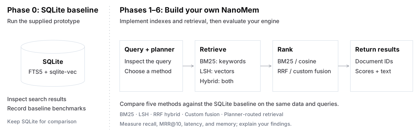 Figure: From a SQLite baseline to your own NanoMem enginePhase 0 uses SQLite FTS5 and sqlite-vec to establish baseline results. A dotted vertical line separates it from Phases 1 through 6: implement a query planner, retrieval, ranking, and results, then benchmark against SQLite.